

Local and long-distance colonization influence the distribution of a species in a fragmented landscape
1 Urban Wildlife Institute, Lincoln Park Zoo, 2001 N. Clark St. Chicago, IL 60614, USA
MF: https://orcid.org/0000-0002-8583-0307
EL: https://orcid.org/0000-0001-5748-6521
SM: https://orcid.org/0000-0003-0275-3885
Kase, A., Fidino, M., Lehrer, E.W., & Magle, S.B. (2025). Local and long-distance colonization influence the distribution of a species in a fragmented landscape. Stacks Journal: 25001. https://doi.org/10.60102/stacks-25001

Abstract photo. A black and white camera trap image from July 2024 of a family of striped skunks in a golf course outside of Chicago, Illinois.
Abstract
Colonization and extinction dynamics are fundamental processes that determine species’ distributions yet nuances of these processes are often overlooked when trying to estimate them. In this study we used dynamic occupancy models to estimate how colonization rates vary when nearby habitat patches are occupied by a species of interest. Our model parameterized colonization as either local (i.e., occurred when a habitat patch was within 2.5 km and was occupied by the species of interest in the previous time step) or long-distance (i.e., occurred when habitat patches within 2.5 km were not occupied by the species of interest in the previous time step). We applied our model to nearly a decade of striped skunk (Mephitis mephitis) camera trap data collected throughout Chicago, Illinois, USA and quantified associations between site-level colonization and persistence rates and proximity to the nearest known stream or river, percentage of developed open space, urbanization, and sampling season (winter, spring, summer, and fall). We found that local colonization was lowest in the fall season and largely controlled by the number of nearby habitat patches occupied by striped skunk. Long-distance colonization was greatest in the fall and positively covaried with developed open space. The probability of skunk persistence was roughly 0.60 adjacent to natural water sources and declined to 0.01 at 14.00 km from natural water sources. Using simulations from our best-fit model we determined that striped skunk occupancy was largely dictated by local colonization and persistence, which collectively accounted for about 80% of the variation in striped skunk occupancy throughout Chicago. Long-distance colonization during the fall season was likely affected by striped skunk offspring dispersing across the landscape. These results demonstrate that by splitting colonization into separate sub-processes, we can more accurately forecast near term changes in species distribution through space and time.
Keywords: Bayesian statistics, camera trap, dynamic occupancy model, colonization, ecological forecasting, striped skunk, urban ecology
Introduction
A central goal in ecology and conservation biology is to determine where species are located (MacArthur 1984, Hunter and Gibbs 2006), particularly given increasingly fragmented and urbanizing landscapes (Mcdonald et al. 2008). Yet, the processes that determine where a species is located—otherwise known as their distribution—are informed by their colonization and extinction rates which makes a species’ distribution dynamic (Yackulic et al. 2015). Two species could have identical distributions but vastly different colonization-extinction dynamics (Evans et al. 2016); thus, inferring processes that drive species distributions from observed distributional patterns can be erroneous (Yackulic et al. 2015). For example, blackbirds (Turdus merula) throughout the Palearctic region were historically forest specialist species that adapted to urban environments over time (Evans et al. 2009). Based on the distribution of blackbirds within cities it was largely believed that individuals from initial urban populations colonized other unoccupied city centers in a leapfrog fashion, but genetic analyses revealed that blackbirds in cities that were later colonized were fully independent from the initial urban blackbird populations (Evans et al. 2009). Understanding colonization-extinction dynamics can be difficult as it not only requires data through possibly long time periods, but colonization and extinction rates can vary through space and time (Fidino and Magle 2017, Hitt and Roberts 2012), with the presence of other species (Fidino et al. 2019, Kleiven et al. 2023), and across scales (Green et al. 2019, Kleiven et al. 2023). Nevertheless, to better predict current and future geographic ranges of species in a rapidly changing world it is critical to understand their colonization-extinction dynamics.
In metapopulation theory, spatial variation in colonization is often accounted for by making this process a function of patch area and isolation (Hanski 1998). While traditional metapopulation models perform well in insular environments like islands—where the space between patches is uninhabitable to a given species—they often fail to capture gradients of habitat suitability or the matrix that characterizes many non-insular environments (Baguette 2004, Howell et al. 2018). Furthermore, local versus long-distance colonization could vary in relative importance for species (Strona 2015). This may be particularly true if a species cannot make long-distance movements (e.g., various land snails) compared to other species that are more mobile (e.g., many bird species, Vélová et al. 2023). Therefore, assuming colonization only varies by patch size and isolation is too simplistic in many terrestrial landscapes because the matrix between patches is not homogenous or inhospitable (Broms et al. 2016).
In terrestrial landscapes, colonization patterns can also be spatially hierarchical such that the first wave of colonization is largely driven by landscape context, whereas subsequent settlement in the surrounding area is controlled by variation in local habitat characteristics (Resetarits and Silberbush, 2016), predation risk at the local or regional scales (Resetarits 2005), and habitat connectivity (Falaschi et al. 2020). Thus, colonization of a patch in the future likely varies due to a species’ current distribution and colonization rates at unoccupied habitat patches located near (i.e., locally) and far from where a species currently exists.
The goal of this study was to quantify the relative contribution of local and long-distance colonization on a species distribution. To do so, we extended the Broms et al. (2016) dynamic occupancy model, allowing us to quantify whether the colonization rate of a species increases if nearby locations are occupied. Furthermore, as a species’ colonization rate is inherently governed by their natural history, we were also interested in accounting for seasonal differences in breeding and subsequent dispersal of offspring. We parameterized this model with nearly a decade of striped skunk (Mephitis mephitis) data collected with camera traps placed throughout Chicago, Illinois, USA. We selected striped skunks for this study because they inhabit a variety of habitat types, are relatively widespread but not ubiquitous on the landscape, are associated with urbanizing environments, and their dispersal distances and home ranges are relatively small compared to other synanthropic mesocarnivores (Bixler and Gittleman 2000, Larivière and Messier 2000, Rosatte et al. 2010, Gallo et al. 2017, Greenspan et al. 2018, Amspacher et al. 2021, Allen et al. 2022). We fitted models that represented six different hypotheses about which factors influenced striped skunk colonization-extinction dynamics (Table 1). Following this, we used simulations from the best-fit model to estimate the relative contributions of local and long-distance colonization on the distribution of striped skunk throughout Chicago. This study demonstrates how colonization dynamics greatly vary throughout an urban region and that both local and long-distance colonization play important parts in determining skunk distributions throughout the city.
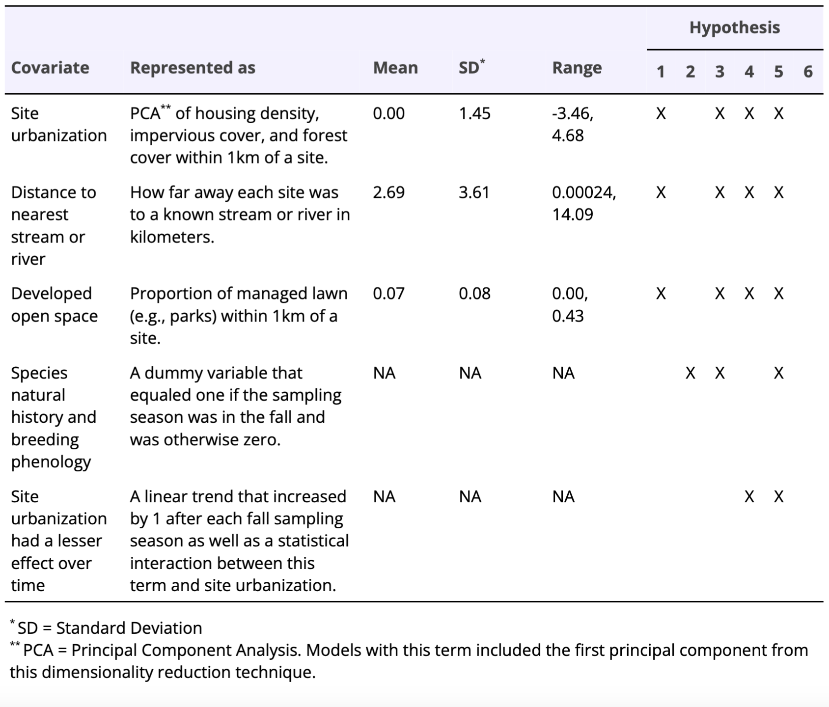
Table 1. Covariates, associated definitions, and summary statistics used to represent our six hypotheses regarding striped skunk occupancy, persistence, and colonization in Chicago, Illinois. Hypotheses for skunk occupancy, colonization, and persistence included testing for the strength of 1) environmental variation, 2) skunk natural history, 3) environmental variation and skunk natural history, 4) environmental variation but urbanization had a lesser effect over time, 5) environmental variation and skunk natural history, but urbanization had a lesser effect over time, or 6) did not vary with any of these variables (i.e., the null model).
Methods and Materials
Biological sampling
This study was part of an ongoing wildlife monitoring survey in Chicago, Illinois (Fidino et al. 2016, Magle et al. 2016). Striped skunk detection data came from sites along four 50-kilometer transects that radiated outwards from the city center to the suburbs (Figure 1, Magle et al. 2016). Sites were in urban greenspace within 2 km of each transect line, and all sites were at a minimum 1 km apart. Examples of greenspace types included natural areas, city parks, golf courses, and cemeteries. If a piece of greenspace was large enough to retain a 1 km distance between camera traps it could contain >1 camera trap sites. We placed one Bushnell motion-triggered infrared Trophy Cam (Bushnell, Overland Park, Kansas, USA) at each site roughly 1-1.5 m above the ground on a tree and pointed at a slight downward angle. We deployed cameras this way to decrease the likelihood of over-triggering cameras by cars on roads adjacent to sites. Cameras were set to normal sensitivity, to take a single photo when triggered, and to pause for 30 seconds after being triggered. Cameras were deployed for roughly 28-day sampling seasons in winter (January), spring (April), summer (July), and fall (October), and were checked once during the middle of a sampling season to change batteries or replace memory cards. A detailed description of site selection, study design, and species identification procedures can be found in Magle et al. (2016).
We included data from 106 sites between 2014 to 2020 in our occupancy models (27 seasons) and held out data from 2021 for out-of-sample validation (4 seasons) to test the dynamic occupancy model’s ability to predict the distribution of striped skunks (i.e., ecological forecasting; Simonis et al. 2021). Over those 27 seasons of training data, four seasons had no data. Three of these seasons (January 2016, July 2016, and October 2018) had no data due to a backlog of images that still needed to be annotated from this long-term study (i.e., the images were collected but our research team has not identified the species in them yet). The fourth season, April 2020, had no data because we could not deploy cameras due to work restrictions associated with the COVID-19 pandemic. This resulted in a total of 23 seasons of training data.
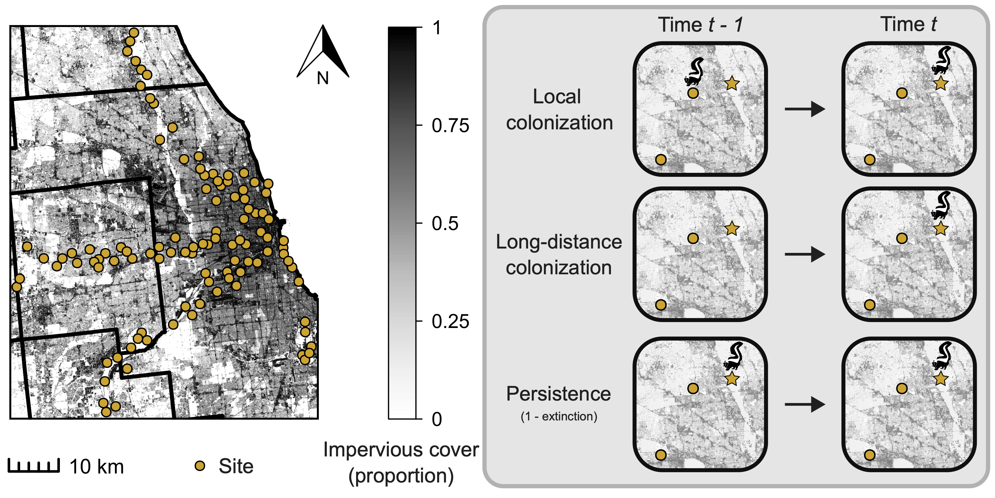
Figure 1. Camera trap sites in urban greenspace throughout the Chicago Metropolitan Area and examples of the different processes estimated throughout our study. For the process examples, focal sites of interest are indicated by stars while sites considered local to a focal site are yellow dots. Sites with skunk present have a skunk above them. Local colonization is the probability the focal site is colonized by skunk at time t when they were present at a nearby (within 2.5 km) site at t-1. Long-distance colonization is the probability the focal site is colonized at time t when the nearby sites are not occupied at t-1. Persistence is the probability skunks occur at the focal site at t-1 and continue to occupy the site at time t, and is the complement of extinction (i.e., persistence = 1 - extinction).
The model
For this model we used variable notation from Broms et al. (2016) and a Bayesian approach to parameterize our model. For i in 1,…,I sites and t in 1,…,T seasons, let zi,t be a Bernoulli random variable that equals 1 if a skunk is present at site i at time t and is zero otherwise. During the first sampling period we have no prior knowledge of site-level occupancy state. Thus, let Ψi be the occupancy probability at site i during the first season

Equation 1.
Initial occupancy can be a function of covariates that affect species occurrence via the logit link, where βψ is a vector of regression coefficients and xiΨ is a vector of conformable covariates, where the first element is 1 to account for the intercept.

Equation 2.
For the remaining sampling periods, we assume a first-order Markov process where occupancy at site i and time t depends on the species location at t-1. Furthermore, following Broms et al. (2016), we split occupancy into three separate processes, which for this study we define as persistence (ϕi,t), long-distance colonization (γi,t), and local colonization (d̅i,t). Persistence (ϕi,t) is the probability that site i remained occupied given the species was present there at time t-1, and is the complement of extinction (ɛi,t) such that ϕi,t = 1 – ɛi,t. Long-distance colonization (γi,t) is the probability site i is colonized if the species was not present at the focal site or any of the neighboring sites at time t-1. Finally, local colonization (d̅i,t) is the probability site i is colonized if the species was not present at the focal site but was present in at least one neighboring site at time t-1. We can estimate these sub-processes from data by conditioning persistence on zi,t-1 and both colonization probabilities on its complement (1- zi,t-1). Further, to differentiate between the two colonization probabilities we use the indicator function INi,t-1, or its complement, which equals 0 unless site i has at least one occupied neighbor at time t-1. Combining these pieces together results in the occupancy probability for site i at time t, which we use in a Bernoulli trial.
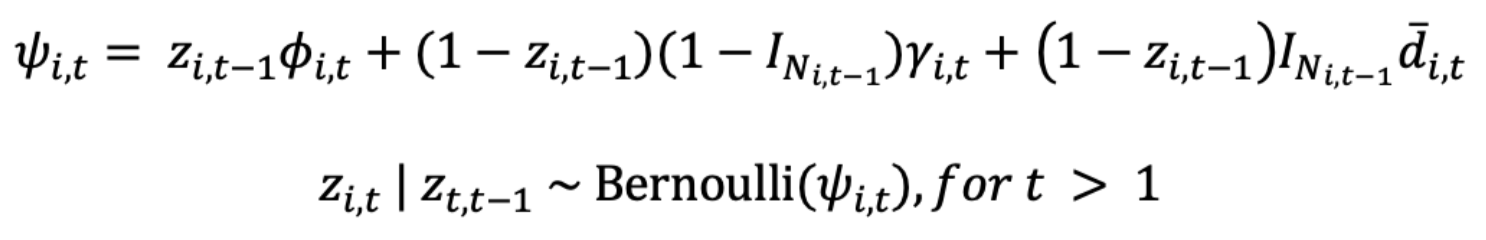
Equation 3.
As with Eqn. 2, both, ϕi,t and γi,t can be made a function of covariates.
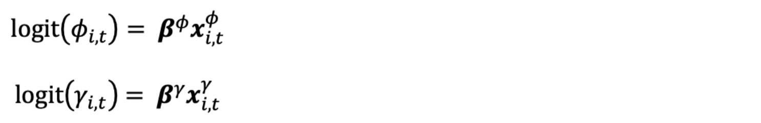
Equation 4.
Where the respective regression coefficients (βϕ and βγ) and vector of conformable covariates (xi,tϕ and xi,tγ) are defined as in Eqn. 2. However, we index these two covariate vectors by both i and t so that persistence and long-distance colonization covariates may vary through space or time.
Local colonization probability depends in part on the number of neighboring occupied sites at t-1

Equation 5.
where zt-1 is a vector of occupancy states across all sites at time t-1, ⊙ is the Hadamard product operator (i.e., element-wise product operator), mi,t-1 is a binary vector of length I that denotes whether each site is considered a neighbor to site i, and di,t is a vector of length I from D, an I x I x T array that contains the probability site i is colonized by each other site. While the Broms et al. (2016) model used the queen’s definition of a neighborhood to determine M, we allowed for a more general sampling structure to determine which sites are neighbors. To do so, let M be an I x I x T binary array that has zeroes on the main diagonal of each MT. Furthermore, let G be an I x I matrix that contains the distance, in meters, between all sites and ht be the distance, in meters, that a species may be expected to disperse during a given sampling period. For many species, ht could be informed by their natural history (e.g., average dispersal distance), which could vary by season. Thus, for all elements within Mt, we determine neighbors as

Equation 6.
where the j index iterates through all the elements of row i and I() is an indicator function that equals 1 if the inequality in Eqn. 6 is true and is otherwise 0. In the event that there is no information on whether a species dispersal distance may vary over time, or if data are collected during one specific time of year (i.e., no seasonal variation), then ht is constant and therefore mi,j,t is also constant across t.
Given Eqn. 6, the element-wise product of zt-1 and mi,t-1 in Eqn. 5 returns a vector that denotes which neighboring sites were occupied at t-1. This product is then multiplied by the transposed vector log(1 – di,t)T, which results in the probability site i is colonized by a species given their presence at some number of neighboring sites (d̅i,t).
Spatial or temporal complexity can also be added to di,t by making them a function of covariates. Following Broms et al. (2016), we use a gradient based colonization model where local colonization was assumed to vary across the landscape and through time. For a single spatial or spatiotemporal covariate, this would be

Equation 7.
Where β0d is the intercept, β1d is a slope term, and xi,td is a vector of length I that contains the difference of a covariate between site i and all other sites, scaled by the distance between the sites
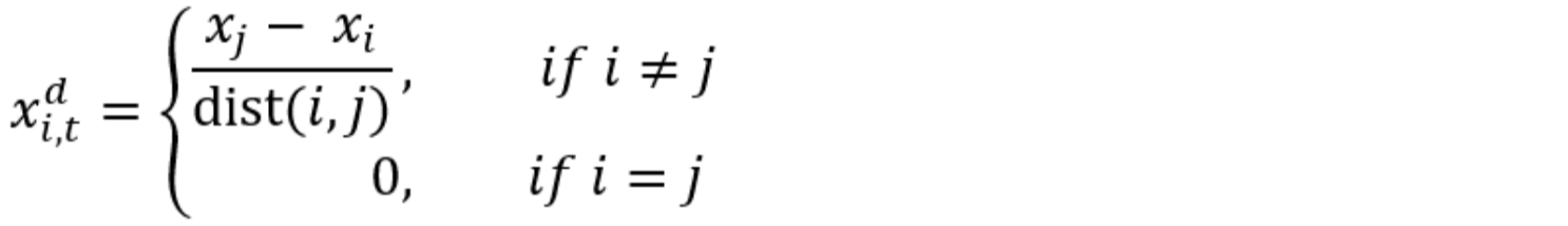
Equation 8.
Temporal covariates are added into di,t differently as there is no gradient for a covariate that does not vary spatially. For example, adding a linear trend to Eqn. 7 would result in: logit(di,t) = β0d + β1d𝒙i,td + β2dt.
For the observational model, let yi,t be the number of secondary sampling units (e.g., days or weeks) a species was detected at site i on sampling period t and ji,t be the total number of secondary sampling units at site i and sampling period t. Assuming that each secondary sampling unit is an i.i.d. Bernoulli trial, we can treat yi,t as a Binomial random variable and estimate the probability of detection, ρi,t, conditional on the presence of the species

Equation 9.
which can be extended to incorporate covariates via the logit link.

Equation 10.
Where the regression coefficients (βρ) and covariates (𝒙i,tρ) are defined similarly to Eqn. 4. Finally, the overall probability of detecting a species at least once given their presence can be derived as 1 – (1 – ρi,t)ji,t, which can be used to determine the overall detection probability across secondary sampling units (Garrard et al. 2008).
Connecting hypotheses to distinct statistical models
For all models, we used 2.5 km as a cutoff to define neighboring sites (Eqn. 6), which falls within the average dispersal distance of 1 – 3 km for striped skunks (Rosatte and Larivière, 2003). Of our six hypotheses, four (H1, H3, H4, and H5) included spatial covariates (Table 1), which we added to every linear predictor of our model (Eqn. 2, 4, 8, and 10). We chose three covariates that past research identified as important determinants of striped skunk distribution: distance to a permanent stream or river, the proportion of open managed lawn within 1 km of a site (i.e., developed open space), and an urbanization metric which was also measured with a 1 km buffer (explained below).
We included site distance to a stream or river because these features function as habitat corridors through urban environments (Douglas and Sadler 2010), and striped skunks use riparian corridors to move across landscapes (Hilty and Merenlender 2004, Frey and Conover 2010). To calculate this metric, we indexed the geographic location of each site to the nearest known stream or river using the sf package in R (Pebesma and Bivand 2023, R Core Team 2023). Stream and river data came from the Illinois Department of Natural Resources (1994). This dataset excluded small (i.e., first-order) streams. The proportion of developed open space was included because striped skunks are omnivorous and acquire much of their dietary items in open grasslands (Greenwood et al. 1999, Gehrt 2004), which in cities can be approximated as developed open space like parks and residential yards. Developed open space data were pulled from the National Land Cover Database (Dewitz et al. 2021), and we used a 1 km buffer around each site to quantify this metric. Finally, urbanization is a variable that is often negatively correlated to the distributions of many medium to large mammals (Magle et al. 2022). We created an urbanization metric with principal component analysis (PCA) using mean tree cover (CMAP 2018), mean impervious cover (CMAP 2018), and mean housing density (Hammer et al. 2004) within a 1 km buffer of each site (Fidino et al. 2016, Magle et al. 2016, Gallo et al. 2017). We retained the first component of this PCA, which explained 69.75% of the variation of the data. Loadings for this metric were tree cover (-0.54), impervious cover (0.64), and housing density (0.54). Therefore, negative values represent areas with more tree cover whereas positive values are areas with more housing density and impervious cover.
In addition to spatial covariates, three hypotheses (H2, H3, and H5) had an additional term related to skunk natural history. We included this term because striped skunks breed between the late winter and early spring and their young disperse in the fall (Rosatte and Larivière, 2003), which can result in higher fall colonization rates (Fidino and Magle 2017). Therefore, the local and long-distance colonization linear predictors (Eqn. 4 and 7) included a temporally varying dummy variable that equaled 1 if a given sampling period occurred in the fall and was otherwise zero.
Finally, two of our hypotheses (H4 and H5, Table 1) had an additional term to evaluate whether striped skunks have become more or less urban over the last decade throughout Chicago. To do so, we included a linear trend that increased by a value of 1 after each fall sampling season throughout Chicago (i.e., the number of fall seasons that have occurred since sampling began). We included this term and its interaction with our site urbanization covariate on the probability of persistence and both colonization probabilities (Eqn. 4 and 8).
Model comparison
We compared models using out-of-sample validation and Brier scores to assess the predictive performance of each model (Brier 1950, Ferro 2007). For a single site across N seasons, the Brier score would be
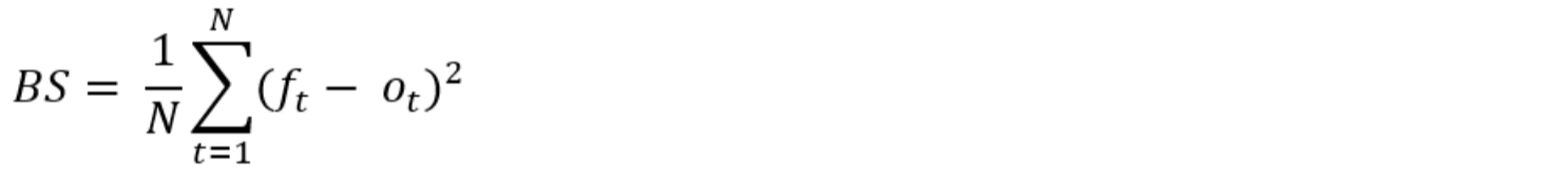
Equation 11.
where N is the number of seasons, ot is whether a skunk was detected (ot = 1) or not (ot = 0), and ft is the forecasted probability of observing this data point, conditional on zt-1. Because our test data is subject to imperfect detection, the forecasted probabilities must be a mixture of occupancy (eqn. 3) and detection (eqn. 10) probabilities. Thus, if ot = 1, then ft was Ψi,t(1 – (1 – ρi,t)ji,t. If ot = 0 then ft was (1 – Ψi,t) + Ψi,t(1 – ρi,t)ji,t. Four seasons of detection data were held out from the initial models and used to test against the model forecasts across Chicago. We calculated Brier scores for each out-of-sample datapoint across the entire posterior distribution of each model, and then compared the median Brier scores among models to evaluate their relative predictive ability.
Prior specification and model fitting
For each model we monitored all logit-scale intercept and slope terms for initial occupancy, local colonization, long-distance colonization, persistence, and detection. All parameters were given uninformative Logistic(0, 1) priors, which are uniform on the probability scale. Each model was run for 50,000 iterations with 10,000 burn-in samples across four chains for a total of 160,000 posterior samples with no thinning. To determine model convergence we inspected posterior samples with traceplots and ensured Gelman-Rubin diagnostics were < 1.1 for all parameters (Gelman et al. 2014). All models were fitted in Program R version 4.4.3 using the nimble package (de Valpine et al. 2017).
We used two methods to quantify the strength of an association between model covariates and each population process. First, we calculated 95% credible intervals and determined whether they overlapped zero. Second, when there was less certainty in the direction of effect based on the bounds of the 95% credible intervals (i.e., they overlapped zero), we calculated the overall probability of an effect as the proportion of the marginal posterior that was greater or less than zero, depending on the direction of effect (Makowski et al. 2019). All data and code to recreate our analysis can be found on GitHub at https://github.com/anna-kase/skunk/.
Quantifying the relative importance of local colonization, long-distance colonization, and persistence on skunk occupancy
To quantify the relative contribution of local colonization, long-distance colonization, and persistence on striped skunk occupancy we simulated skunk distributions across our study area for 12 primary sampling periods across 1000 posterior samples of the best fit model. To do so, we generated a grid of possible habitat patches spaced 1000 m apart. At each point we queried the same spatial covariates used in our model, and scaled each identically to the data used to fit our models. We used rook neighborhoods to determine if a site was nearby so that the maximum number of possible neighbors (4) was similar to the maximum number of neighbors in our data. For the first season, we simulated initial occupancy at each site. Following this, we used the dynamic portion of our best fit model to estimate local colonization, long-distance colonization, or persistence depending on the location of occupied sites during the previous time step. Finally, for each simulation and sampling season we tracked the number of times local colonization, long-distance colonization, and persistence was triggered based on the distribution of skunks in the previous timestep, which we used as a proxy for the relative contribution each of these processes has on skunk distributions throughout Chicago.
Results
Our training data represented 23 primary sampling periods between April 2014 and October 2020. We collected 53,542 camera trap days out of a possible 68,264 sampling days (assuming 106 sites x 23 sampling periods x 28 days of sampling). An average of roughly 70 cameras were operational per season. We detected skunk on 1326 days. The mean naïve occupancy across seasons was 0.19 (min = 0.00, max = 0.37). Overall, striped skunks were detected at least once at 74 of the 106 sites between April 2014 and October 2020.
Based on Brier scores our third hypothesis was most supported (Table 2), which included our three spatial covariates and a life history term that accounted for change in colonization rates over the fall (Table 2). On average, skunk initial occupancy was low (0.09, 95% CI = 0.03, 0.20) and decreased the further a site was from a stream or river (β𝞧river = -1.43, 95% CI = -3.50, -0.06). There was an 0.83 probability that initial occupancy decreased with urbanization (β𝞧urb = -0.32, 95% CI = -1.06, 0.35), and an 0.68 probability initial occupancy was lower with increasing developed open space (β𝞧open space = -0.17, 95% CI = -1.00, 0.56).
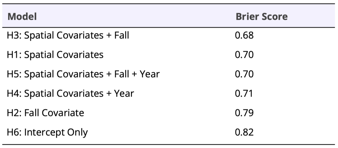
Table 2. Brier scores for each hypothesis model. Brier scores closer to zero indicate a more accurate model forecast.
As with initial occupancy, we found a strong negative relationship between skunk persistence and distance to a stream or river (β𝜙river = -1.35, 95% CI = -2.28, -0.57), though average persistence rates were higher (0.34, 95% = 0.23, 0.45). Persistence was 2.2 times higher (95% CI = 1.36, 4.32) at sites within 100 m of a stream or river than sites ≥3700 m from a stream or river (i.e., roughly 1000 m further than the average distance between a site and a stream or river, Figure 2B). We did not find an association between skunk persistence and urbanization (β𝜙urb = 0.02, 95% CI = -0.29, 0.33) or developed open space (β𝜙open space = 0.09, 95% CI = -0.18, 0.38; Figures 2A,C, respectively).
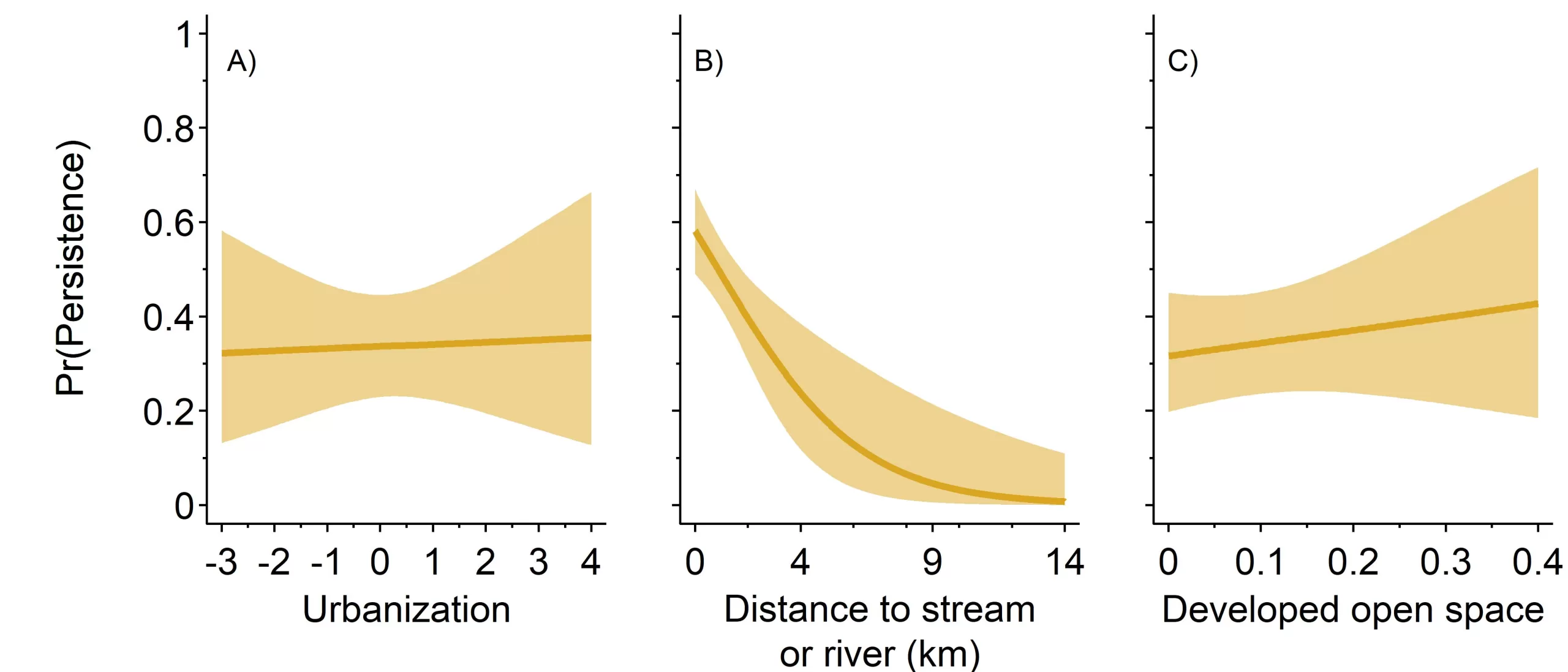
Figure 2. Probability of striped skunk persistence, ϕi,t in relation to three spatial covariates; urbanization, distance to a stream or river (kilometers), and proportion of urban open space. Persistence probabilities were unaffected by site urbanization and proportion of urban open space. Persistence probabilities decreased the further a site was from a stream or river.
On average, long-distance colonization was lower in the spring, summer, and winter (0.07, 95% CI = 0.05, 0.09) than it was in fall (0.17, 95% CI = 0.12, 0.22; βγfall = 0.98, 95% CI = 0.51, 1.45). Furthermore, we found a strong positive relationship between long-distance colonization and developed open space (βγopen space = 0.59, 95% CI = 0.29, 0.93). During the spring, summer, and winter as the proportion of developed open space among sites increased from 0.00 to 0.43 — which represented the range we observed in our data — long-distance colonization increased about 13 times from 0.04 (95% CI = 0.03, 0.06) at 0.00 developed open space to 0.55 (95% CI = 0.23, 0.86) at 0.43 developed open space (Figure 3). Long-distance colonization increased 7.35 times in the fall from 0.10 (95% CI = 0.06, 0.15) at 0.00 open space to 0.76 (95% CI = 0.44, 0.94) at 0.43 open space. There was an 0.95 probability that long-distance colonization decreased with increasing distance to a stream or river (βγwater = -0.26, 95% CI = -0.59, 0.05) and a 0.74 probability long-distance colonization decreased with urbanization (βγurb = -0.08, 95% CI = -0.30, 0.15).
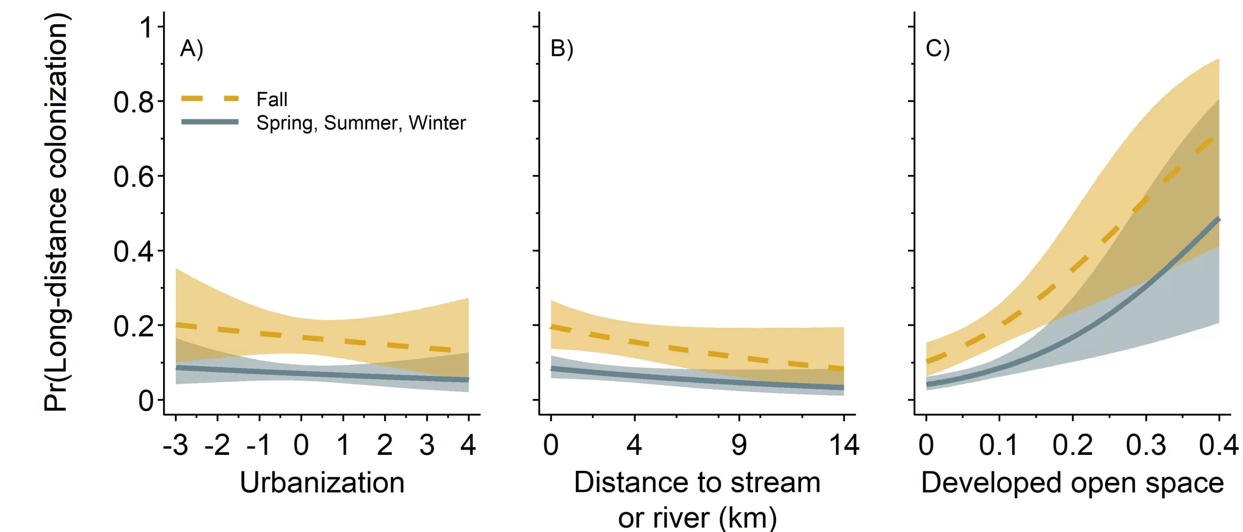
Figure 3. Probability of striped skunk long-distance colonization, γi,t, in relation to three spatial covariates; urbanization, distance to a stream or river (kilometers), and proportion of developed open space, by season. Probability of long-distance colonization was greater in the fall relative to the other three seasons (spring, summer, and winter) for all spatial covariates. Effect sizes for urbanization and distance to a stream or river were lower compared to the proportion of developed open space. As the proportion of developed open space increased the probability of striped skunk long-distance colonization increased.
The average number of neighboring sites across our study was 1.28 (min = 0, max = 4). Overall, we found that the probability of local colonization was, on average, far greater than long-distance colonization except for in the fall (Figure 4, βd̅fall = -0.84, 95% CI = -1.77, -0.03). When skunks occupied one site within 2.5 km of other sites, the probability of local colonization was 0.29 (95% CI = 0.22, 0.37) in the spring, summer, and winter and 0.15 (95% CI = 0.07, 0.27) in the fall (Figure 4). However, the probability of colonization increased as the number of neighboring sites with skunks increased. For a site with four neighboring occupied sites, local colonization was 0.75 (95% CI = 0.63, 0.84) in the spring, summer, and winter and 0.48 (95% CI = 0.24, 0.72) in the fall. We did not find an association between local colonization and urbanization (βd̅urb = 0.08, 95% CI = -1.25, 0.52), distance to a stream or river (βd̅water = -0.19, 95% CI = -2.37, 1.92), or developed open space (βd̅open space = 0.03, 95% CI = -0.53, 0.62).
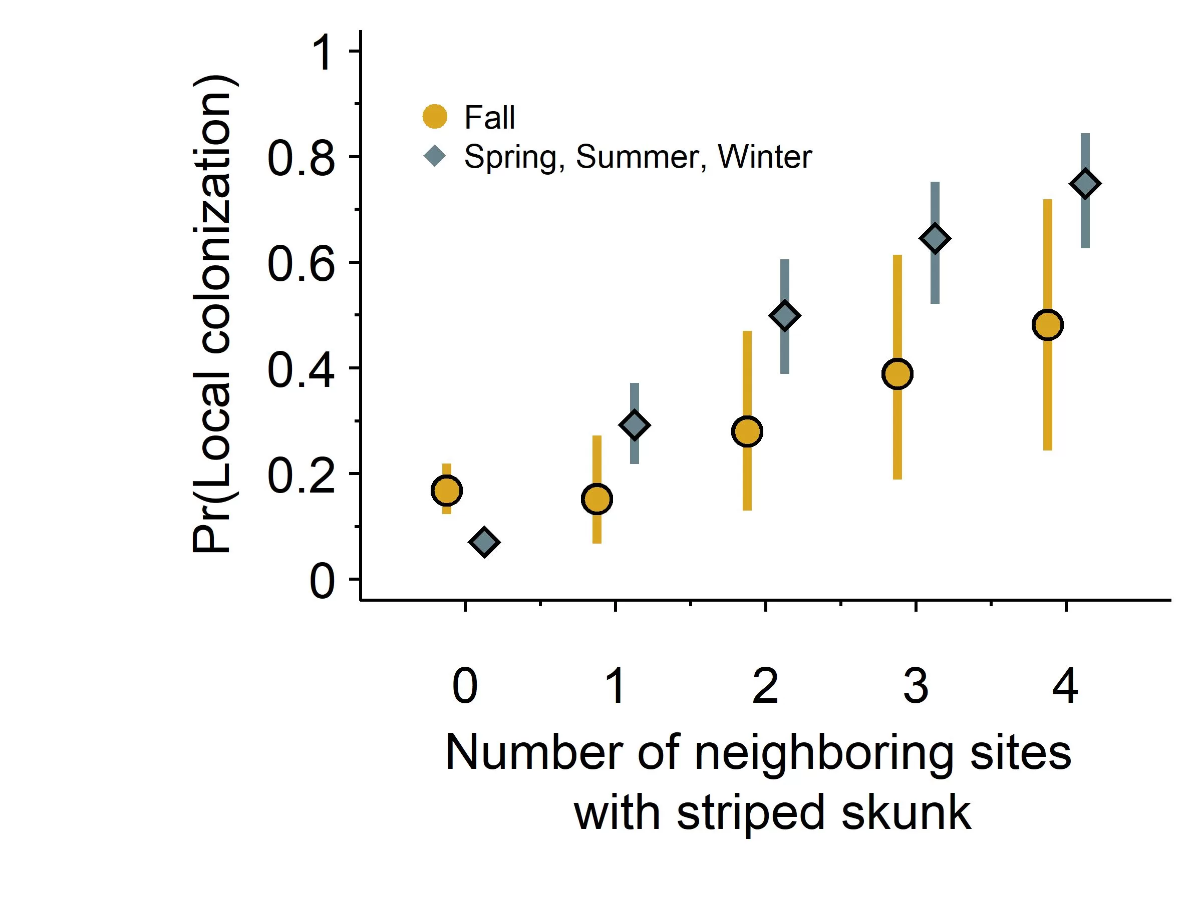
Figure 4. Probability of striped skunk local colonization and the number of occupied neighboring sites by season. As the number of occupied neighbors increased, the probability of local colonization also increased. Overall, local colonization probabilities were greater in the spring, summer, and winter compared to fall. We also included the average probability of long-distance colonization in this figure (i.e., 0 neighboring occupied sites).
On average the daily probability of detecting a skunk given their presence was 0.11 (95% CI = 0.10, 0.12). Thus, given an average 28 days of sampling, the probability skunks were detected at least once given their presence was 0.97 (95% CI = 0.95, 0.97). Skunk detection probability increased with urbanization (βρurb = 0.19, 95% CI = 0.11, 0.27) as well as developed open space (βρopen space = 0.15, 95% CI = 0.08, 0.21). There was only a 0.67 probability that detection probability decreased with distance to water (βρwater = -0.03, 95% CI = -0.16, 0.09).
Based on our simulations we found that local colonization and persistence contributed most to skunk occupancy, particularly in spring, summer, and winter, whereas long-distance colonization generally contributed less (i.e.,<20%) to skunk occupancy (Figure 4). We mapped the average expected occupancy of skunks in our study area using occupancy estimates (n=12 simulated primary sampling periods; Figure 4A), variation in skunk occupancy among simulated primary sampling periods (Figure 4B), and a bivariate choropleth representation of expected occupancy and variation in occupancy (Figure 4C). These results indicated that skunks often occupy the northern and southern suburbs of Chicago, where their occupancy is high and there is low variability in occupancy across seasons. However, the southwestern suburbs also saw intermittent occupancy by skunk, where they had lower occupancy but much higher variability across sampling periods.
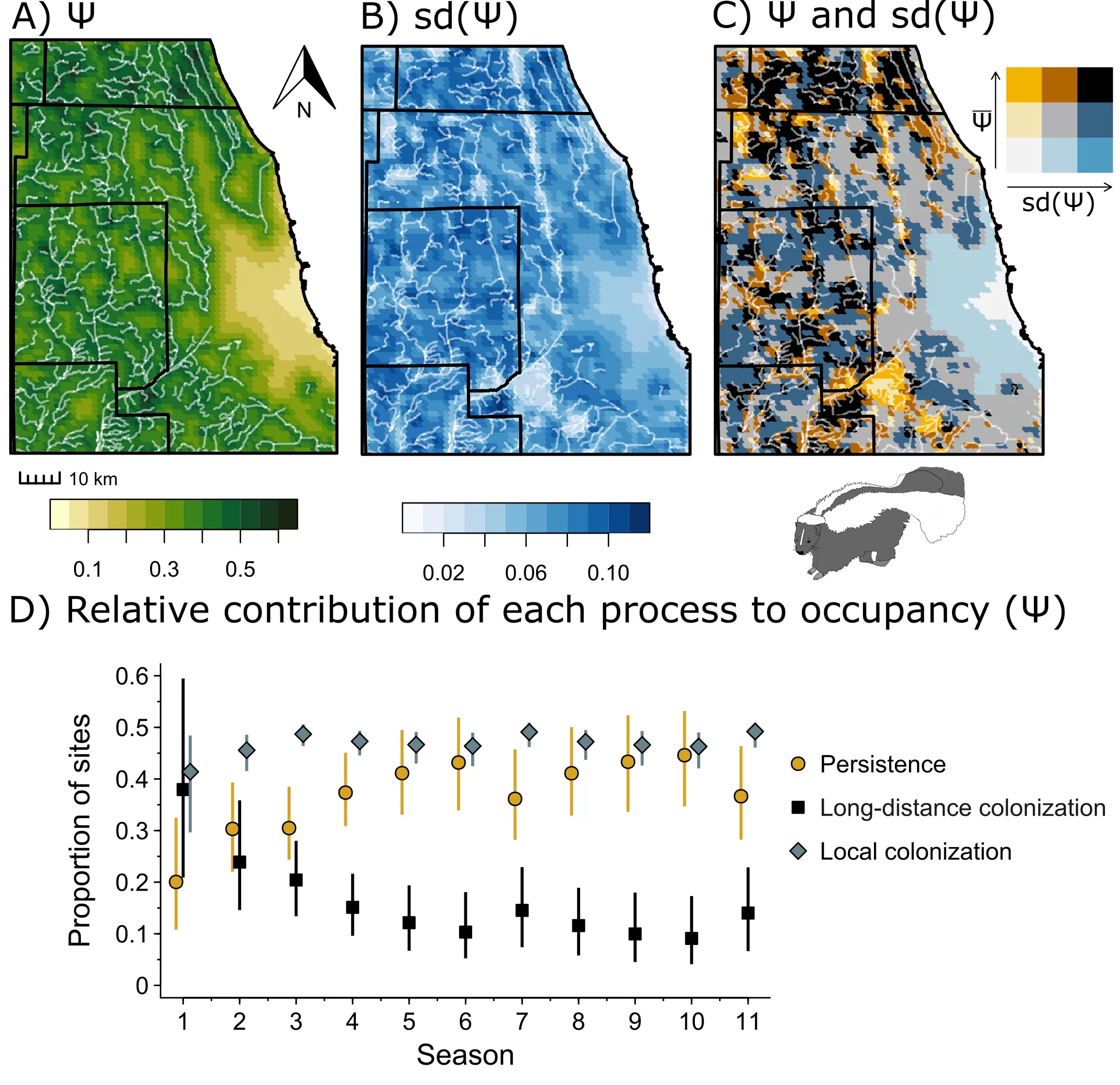
Figure 5. Simulated striped skunk distributions for Chicago, Illinois and surrounding suburbs based on 12 simulated primary sampling periods across 1000 posterior samples of the best fit model (H3). A) Average expected occupancy probability. B) Standard deviation of average occupancy probability across simulated primary sampling periods where higher values indicate areas with greater temporal variability in occupancy. C) Bivariate choropleth representation of expected occupancy and variation in occupancy. This sub-figure can be used to see, for example, areas that are high in occupancy and low in temporal variability, which indicates locations that skunks regularly occupy. D) Relative contribution of persistence, long-distance colonization, and local colonization to striped skunk occupancy.
Discussion
Overall, colonization processes were driven primarily by striped skunks moving into neighboring unoccupied habitat patches between seasons (i.e., local colonization in this study). However, in the fall, long-distance colonization also played an important role in the spatial distribution of occupied habitat patches. These two findings align with our third hypothesis, i.e., striped skunk occupancy is governed by environmental variation and their natural history. With respect to skunk natural history, female striped skunks are philopatric and remain near natal dens while males may disperse farther in the fall (Talbot et al. 2012, Brashear et al. 2015). Thus, young female striped skunks are likely establishing dens in areas surrounding natal locations, corresponding to local colonization in our model. Male skunks are largely intolerant of other males and will typically den alone or visit communally denning females (Theimer et al. 2016). This creates a demand for non-competitive domains potentially pushing males farther to colonize distant areas and contributing to the increased probability of long-distance colonization in the fall observed in this study. Unfortunately, because striped skunks are not sexually dimorphic, we could not evaluate this hypothesis with our camera trap data. Nevertheless, splitting colonization into separate sub-processes in a dynamic occupancy model provided unique insights into processes affecting skunk spatial distribution. This division of colonization processes may be particularly useful for species whose dispersal processes are not fully known, as is the case for many species.
In addition to being higher in the fall, long-distance colonization was also positively associated with the amount of developed open space like city parks and yards. Developed open space is favorable for striped skunks as invertebrate prey items are typically abundant in managed lawns that characterize these areas (Rosatte et al. 2010). Additionally, developed open space may provide a bounty of anthropogenic resources like water, discarded food scraps, or pet food (Rosatte et al. 2010). As areas with greater-than-average amounts of developed open space are highly likely to be colonized by skunks, these areas may function as staging points for further colonization into adjacent habitat patches. Areas with abundant developed open space also had high skunk persistence rates, especially if they were near streams or rivers. Thus, these findings indicate that developed open space is an important feature for understanding and predicting population level processes for this species.
One critical aspect affecting animal distributions we could not portray in our model was the relationship between local or long-distance colonization events and any source-sink dynamics for skunks throughout Chicago. In a source-sink metapopulation, both high-quality (i.e., source) and low-quality (i.e., sink) habitat patches help maintain population stability (Foppen et al. 2000). Theoretically, sink habitats can function as refuges where individuals persist so long as the population remains connected to other populations (Howe et al. 1991). In turn, sink habitats can increase a species’ overall abundance on the landscape and increase the survival of dwindling metapopulations (Howe et al.1991). As it may be possible to identify source habitat from species distribution models (Şen et al. 2024), we suggest that these areas are likely located along streams outside of the city of Chicago, which have relatively high and stable occupancy patterns through time (Figure 4). What we are uncertain of, however, is whether local or long-distance colonization contribute more towards this species residing in sink habitats, or what qualities these habitats possess. While we do know local colonization occurs more often, demographic or genetic studies conducted both near and far from skunk source habitats could further clarify the roles of local and long-distance colonization on source-sink dynamics for this metapopulation (Minnie et al. 2018).
While we attributed the lack of environmental variation in local colonization to the natural history of striped skunks, other factors may have influenced this outcome. First, while our camera transects covered a broad range of environmental variation from downtown Chicago outward to 50 km, not every potential habitat patch for skunks was surveyed. Thus, there were undoubtedly unsampled habitat patches where skunks resided adjacent to monitored ones, which likely influenced how we should interpret long-distance colonization in our model. It may be that a colonization event detected on our cameras was not truly long-distance. Thus, it may be safer to assume that long-distance colonization is effectively random colonization, as it could have occurred from any location other than neighboring habitat patches that were surveyed, regardless of distance. As always, it is critical to consider how a given study design may impact model interpretation.
Additionally, we potentially failed to find effects of environmental variation on local colonization due to how the model was constructed. We used a gradient-based approach in this analysis, which compared differences in the environmental covariates between a site of interest and its surrounding neighbors (eqn. 8). It may be that skunks do not compare the relative quality of habitat patches, which is what our gradient based approach quantified. For others interested in using this modeling framework we suggest two ways to adjust local colonization if the gradient-based approach is insufficient. First, the model could be simplified by using a homogeneous local colonization rate by removing environmental covariates from this level of the model (i.e., an intercept-only model for local colonization). Such a specification would still allow for changes in local colonization if the number of occupied neighboring patches differs but assumes no environmental variation in this rate. Second, local colonization could be extended to include the actual local habitat covariate values themselves, instead of or in addition to the differences of these variables between sites (Broms et al. 2016). While the current model formulation we used represents a middle ground in terms of complexity, numerous options are available to those interested in better tailoring this model to a species’ natural history or a specific study area.
Even though the goal of this study was to uncover the relative roles local and long-distance colonization have on a species distribution, our results could also be applied to mitigate human-wildlife conflict. Striped skunks are generally considered an undesirable species to humans as they can damage property, particularly lawns and golf courses with their foraging activity (O’Donnell and VanDruff 1983, Rosatte et al. 2010). Striped skunks also have the reputation of defensively spraying domesticated dogs, leading to increased wariness from pet owners (O’Donnell and VanDruff 1983, Rosatte et al. 2010), and can be a public health concern as skunks may carry diseases that could affect people and pets like rabies (Blanton et al. 2010). Therefore, by determining where striped skunks are and where they might colonize and persist on the landscape appropriate management actions may be taken, from posting informational signage in public spaces to identifying areas to monitor for disease concerns.
Management strategies could further be tailored depending on whether skunk occupancy is high, low, frequent, or intermittent. For example, educational programs may only be necessary in areas where skunk occupancy is either low or intermittent as people living there may be less familiar with the species. Conversely, local ordinances that could reduce the likelihood of skunk denning on people’s property may be used in conjunction with educational programs in parts of the city where skunk occupancy is high and frequent (Merkle et al. 2011). These methods of mitigating wildlife conflict can be applied to other species and may be particularly useful for other synanthropic species.
For those interested in using this modeling approach with their own data, it is important to consider the scarcity of the study species on the landscape and the amount of data needed to parameterize this model. This is because there must be sufficient data for all processes to estimate their associated parameters (Mckann et al. 2013). For example, if only a small number of long-distance colonization events are observed, estimating spatial variation in this process would be difficult. In our study striped skunks were relatively rare. Thus, our analysis required a larger sample size, as rare species in general have low detection probabilities (Kowalski et al. 2015, Fidino et al. 2020). To overcome this, we leveraged nearly a decade-long time series that collected samples four times per year. While we were able to achieve an average 0.97 total detection probability with our study design, low species detection probabilities can make it difficult to accurately predict ecological processes (Neilson et al. 2018, Stewart et al. 2018, Emmet et al. 2021). While we do not suggest that a decade’s worth of data is required to fit this model, we encourage others to strongly consider their sample size with respect to the number of transitions they may see between time periods (i.e., unoccupied to occupied, and vice versa). As dynamic occupancy models are already data hungry, this version, which further extends the colonization process, is even more so (Mckann et al. 2013).
Although we identified a top predictive model, the Brier score of our best fit model indicated there was substantial room for improvement. Undoubtedly, there was unexplored heterogeneity in skunk distribution that could be identified by considering additional covariates, their interactions, non-linear relationships, or spatiotemporal autocorrelation (Tredennick et al. 2021). Adding these terms and increasing model complexity is challenging, however, as many ecological time-series do not have sufficient data to estimate the effect of many covariates at once (Teller et al. 2016, Tredennick et al. 2021). Conversely, the distribution of skunks may have changed between our training (2014 – 2020) and test (2021) data, and so the forecasts did not perform well on the test data (Simonis et al. 2021). Regardless, our best fit model outperformed a null model, suggesting some utility in forecasting skunk distributions.
Overall, this modelling framework proved useful to disentangle species distributional patterns from population processes. Using a long-term camera-trapping dataset, we show that the relative contribution of local versus long-distance colonization on spatial distribution differs for striped skunks. By using species detection data to evaluate colonization behavior in a more nuanced way, we provide a valuable tool for conservation and management that can help elucidate the natural history of wildlife in fragmented habitats.
Acknowledgments
Funding was provided by the Abra Prentice-Wilkin Foundation and the EJK Foundation. We thank all eight reviewers for their comments, which greatly increased the clarity of this manuscript.
Author Contributions
Anna Kase: conceptualization, writing – review & editing, writing – original draft, Formal analysis.
Mason Fidino, conceptualization, writing – review & editing, writing – original draft, Formal analysis, data curation.
Elizabeth Lehrer: writing – review & editing, data curation.
Seth Magle: writing – review & editing, data curation, project administration.
Data Availability
All data and code are available at https://github.com/anna-kase/skunk
Transparent Peer Review
Results from the Transparent Peer Review can be found here.
Recommended Citation
Kase, A., Fidino, M., Lehrer, E.W., & Magle, S.B. (2025). Local and long-distance colonization influence the distribution of a species in a fragmented landscape. Stacks Journal: 25001. https://doi.org/10.60102/stacks-25001
References
Allen, Maximilian L., Austin M. Green, and Remington J. Moll. 2022. “Habitat productivity and anthropogenic development drive rangewide variation in striped skunk (Mephitis mephitis) abundance.” Global Ecology and Conservation 39: e02300.
Amspacher, Katelyn, F. Agustín Jiménez, and Clayton Nielsen. 2021. “Influence of habitat on presence of striped skunks in Midwestern North America.” Diversity 13, no. 2: 83.
Baguette, Michel. 2004. “The classical metapopulation theory and the real, natural world: a critical appraisal.” Basic and Applied Ecology 5 no. 3: 213-224.
Bixler, Andrea, and John L. Gittleman. 2000. “Variation in home range and use of habitat in the striped skunk (Mephitis mephitis).” Journal of Zoology 251 no. 4: 525-533.
Blanton, Jesse D., Dustyn Palmer, and Charles E. Rupprecht. 2010. “Rabies surveillance in the United States during 2009.” Journal of the American Veterinary Medical Association 237, no. 6: 646-657.
Brashear, Wesley A., Leren K. Ammerman, and Robert C. Dowler. 2015. “Short-distance dispersal and lack of genetic structure in an urban striped skunk population.” Journal of Mammalogy 96 no. 1: 72-80.
Brier, Glenn W. 1950. “Verification of forecasts expressed in terms of probability.” Monthly weather review 78, no. 1: 1-3.
Broms, Kristin M., Melvin B. Hooten, Devin S. Johnson, Res Altwegg, and Loveday L. Conquest. 2016. “Dynamic occupancy models for explicit colonization processes.” Ecology 97 no. 1: 104-204.
Chicago Metropolitan Agency for Planning Data Hub (CMAP). 2018. “High Resolution Land Cover, NE Illinois and NW Indiana.” Retrieved 10 August 2021 from https://datahub.cmap.illinois.gov/ 10 of 12 FIDINO ET AL. dataset/high-resolution-land-cover-ne-illinois-and-nw-indiana2010.
Dewitz, J., and U.S. Geological Survey, 2021, National Land Cover Database (NLCD) 2019 Products (ver. 2.0, June 2021): U.S. Geological Survey data release.
Douglas, Ian, and Jonathan P. Sadler. 2010. “Urban wildlife corridors.” The Routledge Handbook of Urban Ecology: 274.
Emmet, Robert L., Robert A. Long, and Beth Gardner. 2021. “Modeling multi-scale occupancy for monitoring rare and highly mobile species.” Ecosphere 12 no. 7: e03637.
Evans, Karl L., Kevin J. Gaston, Alain C. Frantz, Michelle Simeoni, Stuart P. Sharp, Andrew McGowan, Deborah A. Dawson et al. 2009. “Independent colonization of multiple urban centres by a formerly forest specialist bird species.” Proceedings of the Royal Society B: Biological Sciences 276, no. 1666: 2403-2410.
Evans, Margaret, Cory Merow, Sydne Record, Sean McMahon, and Brian Enquist. 2016. “Towards process-based range modeling of many species.” Trends in Ecology and Evolution 31 no. 11: 860-871.
Ferro, Christopher A. T. 2007. “Comparing probabilistic forecasting systems with the Brier score.” Forecasting 22 no. 5: 1076-1088.
Falaschi, M., Giachello, S., Lo Parrino, E., Muraro, M., Manenti, R., and Ficetola, G. F. 2020. “Long‐term drivers of persistence and colonization dynamics in spatially structured amphibian populations.” Conservation Biology, 35(5), 1530-1539.
Fidino, Mason, Elizabeth W. Lehrer, and Seth B. Magle. 2016. “Habitat dynamics of the Virginia opossum in a highly urban landscape.” The American Midland Naturalist 175 no. 2: 155-167.
Fidino, Mason, and Seth B. Magle. 2017. “Using Fourier series to estimate periodic patterns in dynamic occupancy models.” Ecosphere 8 no. 9: e01944.
Fidino, Mason, Juniper L. Simonis, and Seth. B. Magle. 2019. “A multistate dynamic occupancy model to estimate local colonization-extinction rates and patterns of co-occurrence between two or more interacting species.” Methods in Ecology and Evolution 10 no. 2: 233-244.
Fidino, Mason, Gabriella R. Barnas, Elizabeth W. Lehrer, Maureen H. Murray, and Seth B. Magle. 2020. “Effect of lure on detecting mammals with camera traps.” Wildlife Society Bulletin 44 no. 3: 543-552.
Frey, Shandra Nicole, and Michael R. Conover. 2010. “Effects of waterfowl hunting on raccoon movements.” Human-Wildlife Interactions 4 no. 1: 95-102.
Foppen, Ruud PB, J. Paul Chardon, and Wendy Liefveld. 2000. “Understanding the role of sink patches in source‐sink metapopulations: Reed Warbler in an agricultural landscape.” Conservation Biology 14, no. 6: 1881-1892.
Gallo, Travis, Mason Fidino, Elizabeth W. Lehrer, Seth B. Magle. 2017. “Mammal diversity and metacommunity dynamics in urban green spaces: implications for urban wildlife conservation.” Ecological Applications 27 no. 8: 2330-2341.
Garrard, Georgia E., Sarah A. Bekessy, Micheal A. McCarthy, and Brendan A. Wintle. 2008. “When have we looked hard enough? A novel method for setting minimum survey effort protocols for flora surveys.” Austral Ecology 33, no. 8: 986-998.
Gehrt, Stanley D. 2004. “Ecology and management of striped skunks, raccoons, and coyotes in urban landscapes.” In People and Predators: From Conflict to Coexistence. Fascione, Nina, Aimee Delach, and Martin E. Smith (eds). Island Press.
Gelman, Andrew, John B. Carlin, Hal S. Stern, David B. Dunson, Aki Vehtari, and Donald B. Rubin. 2014. Bayesian Data Analysis. Boca Raton, FL: CRC Press
Green, Adam W., David C. Pavlacky Jr., and T. Luke George. 2019. “A dynamic multi-scale occupancy model to estimate temporal dynamics and hierarchical habitat use for nomadic species.” Ecology and Evolution 9 no. 2: 793-803.
Greenspan, Evan, Clayton K. Nielsen, and Kevin W. Cassel. 2018. “Potential distribution of coyotes (Canis latrans), Virginia opossums (Didelphis virginiana), striped skunks (Mephitis mephitis), and raccoons (Procyon lotor) in the Chicago metropolitan area.” Urban Ecosystems 21: 983-997.
Greenwood, Raymond J., Alan B. Sargeant, James L. Piehl, Deborah A. Buhl, and Bruce A. Hanson. 1999. “Foods and foraging of prairie striped skunks during the avian nesting season.” Wildlife Society Bulletin 27 no. 3: 823-832.
Hammer, Roger B., Susan I. Stewart, Richelle L. Winkler, Volker C. Radeloff, and Paul R. Voss. 2004. “Characterizing Dynamics Spatial and Temporal Residential Density Patterns from 1940–1990 across the North Central United States.” Landscape and Urban Planning 69 no. 2-3: 183–99.
Hanski, Ilkka. 1998. “Metapopulation dynamics.” Nature 396: 41-49.
Hilty, Jodi A., and Adina M. Merenlender. 2004. “Use of riparian corridors and vineyards by mammalian predators in Northern California.” Conservation Biology 18 no. 1: 126-135.
Hitt, Nathaniel, and James Roberts. 2012. “Hierarchical spatial structure of stream fish colonization and extinction.” Oikos 121: 127-137.
Howe, Robert W., Gregory J. Davis, and Vincent Mosca. 1991. “The demographic significance of ‘sink’ populations.” Biological Conservation 57, no. 3: 239-255.
Howell, Paige E., Erin Muths, Blake R. Hossack, Brent H. Sigafus, and Richard B. Chandler. 2018. “Increasing connectivity between metapopulation ecology and landscape ecology.” Ecology 99 no. 5: 1119-1128.
Hunter Jr, M. L., & Gibbs, J. P. (2006). Fundamentals of conservation biology. John Wiley & Sons.
Illinois Department of Natural Resources. 1994. “Streams and Shorelines in Illinois.” Edition 20040401 from ISGS GIS Database.
Kleiven, Eivind Flittie, Frédéric Barraquand, Olivier Gimenez, John-
André Henden, Rolf Anker Ims, Eeva Marjatta Soininen, and Nigel Gilles Yoccoz. 2023. “A dynamic occupancy model for interacting species with two spatial scales.” Journal of Agricultural, Biological and Environmental Statistics 28: 466-482.
Kowalski, Bart, Fred Watson, Corey Garza, and Bruce Delgado. 2015. “Effects of landscape covariates on the distribution and detection probabilities of mammalian carnivores.” Journal of Mammalogy 96 no. 3: 511-521.
Larivière, Serge, and François Messier. 2000. “Habitat selection and use of edges by striped skunks in the Canadian prairies.” Canadian Journal of Zoology 78 no. 3: 366-372.
MacArthur, R. H. 1984. Geographical ecology: patterns in the distribution of species. Princeton University Press.
Makowski, Dominique, Mattan S. Ben-Shachar, and Daniel Lüdecke. 2019. “bayestestR: Describing effects and their uncertainty, existence and significance within the Bayesian framework.” Journal of Open Source Software 4, no. 40: 1541.
Magle, Seth B., Elizabeth W. Lehrer, and Mason Fidino. 2016. “Urban mesopredator distribution: examining the relative effects of landscape and socioeconomic factors.” Animal Conservation 19 no. 2: 163-175.
Magle, Seth B., Mason Fidino, Heather A. Sander, Adam T. Rohnke, Kelli L. Larson, Travis Gallo, … & Christopher J. Schell. 2022. “Wealth and urbanization shape medium and large terrestrial mammal communities.” Global Change Biology 27 no. 21: 5446-5459.
McDonald, R. I., Kareiva, P., & Forman, R. T. 2008. “The implications of current and future urbanization for global protected areas and biodiversity conservation.” Biological conservation, 141(6), 1695-1703.
McKann, Patrick C., Brian R. Gray, and Wayne E. Thogmartin. 2013. “Small sample bias in dynamic occupancy models.” The Journal of Wildlife Management 77 no. 1: 172-180.
Merkle, J. A., P. R. Krausman, N. J. Decesare, and J. J. Jonkel. 2011. “Predicting Spatial Distribution of Human–Black Bear Interactions in Urban Areas.” The Journal of Wildlife Management 75 (5): 1121–7.
Minnie, Liaan, Andrzej Zalewski, Hanna Zalewska, and Graham IH Kerley. 2018. “Spatial variation in anthropogenic mortality induces a source–sink system in a hunted mesopredator.” Oecologia 186: 939-951.
Neilson, Eric W., Tal Avgar, A. Cole Burton, Kate Broadley, and Stan Boutin. 2018. “Animal movement affects interpretation of occupancy models from camera-trap surveys of unmarked animals.” Ecosphere 9 no. 1: e02092.
O’Donnell, Machael a., and Larry W. VanDruff. 1983. “Wildlife conflicts in an urban area: occurrence of problems and human attitudes toward wildlife.” In Decker, D.J. (ed.), The First Eastern Wildlife Damage Control Conference (pp. 315-323). Ithaca, NY: Cornell University.
Pebesma, Edzer, and Roger Bivand. 2023. Spatial Data Science: With applications in R. Chapman and Hall/CRC.
R Core Team. 2023. “R: A Language and Environment for Statistical Computing.” R Foundation for Statistical Computing, Vienna, Austria.
Resetarits Jr, W. J. 2005. “Habitat selection behaviour links local and regional scales in aquatic systems.” Ecology Letters, 8(5), 480-486.
Resetarits Jr, W. J., and Silberbush, A. 2016. “Local contagion and regional compression: habitat selection drives spatially explicit, multiscale dynamics of colonisation in experimental metacommunities.” Ecology Letters, 19(2), 191-200.
Rosatte, Richard, Kirk Sobey, Jerry W. Dragoo, and Stanley D. Gehrt. 2010. “Striped Skunks and Allies (Mephitis spp.). in Stanley D. Gehrt, Seth P. D. Riley, and Brian L. Cypher (eds) Urban Carnivores. The Johns Hopkins University Press, 97-109.
Rosatte, Richard C. and Serge Larivière. 2003. Skunks, p. 692 – 707. In: G. A. Feldhamer, B. C. Thompson and J.A. Chapman (eds.). Wild mammals of North America: biology, management, and conservation. 2nd ed. John Hopkins University Press, Baltimore, M.D.
Şen, Bilgecan, Christian Che‐Castaldo, and H. Reşit Akçakaya. 2024. “The potential for species distribution models to distinguish source populations from sinks.” Journal of Animal Ecology 93, no. 12: 1924-1934.
Simonis, Juniper L., Ethan P. White, and SK Morgan Ernest. 2021. “Evaluating probabilistic ecological forecasts.” Ecology 102, no. 8: e03431.
Stewart, Frances E.C., Jason T. Fisher, A. Cole Burton, and John P. Volpe. 2018. “Species occurrence data reflect the magnitude of animal movements better than the proximity of animal space use.” Ecosphere 9 no. 2: e02112.
Strona, Giovanni. 2015. “A spatially explicit model to investigate how dispersal/colonization tradeoffs between short and long distance movement strategies affect species ranges.” Ecological Modelling 297: 80-85.
Talbot, Benoit, Dany Garant, Sébastien Rioux Paquette, Julien Mainguy, and Fanie Pelletier. 2012. “Lack of genetic structure and female-specific effect of dispersal barriers in a rabies vector, the striped skunk (Mephitis mephitis).” PLOS ONE 7 no. 11: e49736.
Teller, B. J., P. B. Adler, C. B. Edwards, G. Hooker, R. E. Snyder, and S. P. Ellner. 2016. Linking demography with drivers: climate and competition. Methods in Ecology and Evolution 7: 171–183.
Theimer, Tad C., Jesse M. Maestas, and David L. Bergman. 2016. “Social contacts and den sharing among suburban striped skunks during summer, autumn, and winter.” Journal of Mammalogy 97 no. 5: 1272-1281.
Tredennick, A. T., Hooker, G., Ellner, S. P., & Adler, P. B. 2021. “A practical guide to selecting models for exploration, inference, and prediction in ecology.” Ecology, 102(6), e03336.
de Valpine, Perry, Daniel Turek, Christopher J. Paciorek, Clifford Anderson-Bergman, Duncan Temple Lang, and Rastislav Bodik. 2017. “Programming with models: writing statistical algorithms for general model structures with NIMBLE.” Journal of Computational and Graphical Statistics 26 no. 2: 403-413.
Vélová, Lucie, Adam Véle, Alena Peltanová, Lenka Šafářová, Rosa Menendéz, and Jakub Horák. 2023. “High-, medium-, and low-dispersal animal taxa communities in fragmented urban grasslands.” Ecosphere 14 no. 2: e4441.
Yackulic, Charles, James Nichols, Jancie Reid, and Ricky Der. 2015. “To predict the niche, model colonization and extinction.” Ecology 96 no. 1: 16-23.
Accepted by 8 of 8 reviewers
Open Access
Peer-Reviewed
Creative Commons
Accepted: 5 March 2025
Published: 24 March 2025
Funding Information: Funding was provided by the Abra Prentice-Wilkin Foundation and the EJK Foundation.
Conflicts of Interest: The authors declare no conflicts of interest.
© 2025 Kase et al. Stacks Journal


