

Spatial and temporal activity of wildlife on and surrounding cannabis farms
1 University of California, Berkeley, Department of Environmental Science, Policy, and Management, Berkeley, CA, USA.
PPS: https://orcid.org/0000-0002-1738-0471
2 The Cannabis Research Center at Berkeley, University of California Berkeley, Berkeley, CA, USA.
BRG: https://orcid.org/0000-0001-8015-7494
JSB: https://orcid.org/0000-0002-3973-5632
3 Department of Forestry and Environmental Resources, North Carolina State University, Raleigh, NC, USA.
Parker-Shames, P., Goldstein, B.R., & Brashares, J.S. (2024). Spatial and temporal activity of wildlife on and surrounding cannabis farms. The Stacks: 24003. https://doi.org/10.60102/stacks-24003

Abstract photo. Image of a mountain lion on a cannabis farm, captured on remote camera for this study.
Abstract
This study introduces a model to assess wildlife space use and activity patterns, demonstrated in the context of small-scale cannabis cultivation in the western United States. We examined local wildlife space use and diel activity patterns at a gradient of distances to active small-scale (<1 acre) private-land outdoor cannabis farms. We used data from 149 cameras on and surrounding eight cannabis farms in the Klamath-Siskiyou Ecoregion in southern Oregon, collected between 2018–2019. Using single species occupancy analyses, we assessed how cannabis production influenced occupancy (defined here as space use) and detection (defined here as a combination of detectability and space use intensity) of 13 wild and one domestic animal species in our study area. We also developed and used multi-state diel models on nine of these species to assess degree of nocturnality along a gradient of distances to cannabis production. We found that 8 of 14 species in single-species models responded to presence of cannabis farms in either their use of space or in intensity of use, and 6 of 9 species in the diel models altered nocturnality in relation to cannabis production, though the responses for both models were species-specific. Our results suggest three main types of responses to cannabis production: avoidance, attraction, and mixed. Some species (e.g., black-tailed deer) used space near cannabis farms less, and became more nocturnal closer to farms. Other species (e.g., gray fox) increased space use near cannabis farms, and became less nocturnal closer to farms. Finally, some species displayed behavioral tradeoffs (e.g., California and mountain quail), and displayed site-specific patterns of use. Additionally, our results suggest that cannabis development may trigger opposing diel responses in larger and smaller bodied animals, where species such as black bear or black-tailed deer become more nocturnal close to farms, but other smaller species become less nocturnal. The success of our modeling approach in revealing nuanced wildlife responses to land use change highlights its potential utility for evaluating novel disturbances and informing mitigation measures.
Keywords: agricultural frontier, camera trap, diel models, hierarchical Bayesian models, human disturbance, occupancy models, rural development, working lands
Introduction
Wildlife response to disturbance across landscape gradients is complex, as animals adjust behaviorally in both space use and activity patterns (e.g., physically avoiding a disturbance, or becoming more nocturnal around disturbance sources) (Frid and Dill 2002; Gaynor et al. 2018; Van Scoyoc et al. 2023). Disturbances are heavily context-dependent, affecting species differently — attracting some or deterring others — and leading to contractions or expansions in species assemblages and interactions (Fidino et al. 2021; Padilla and Sutherland 2021; Van Scoyoc et al. 2023; Mendenhall et al. 2014; Schmitz, Krivan, and Ovadia 2004; Y. Wang, Smith, and Wilmers 2017). Such changes, particularly if they involve keystone species, can influence ecosystem function (Estes, Terborgh, and Brashares 2011; Power et al. 1996; Prugh et al. 2009). In turn these responses can impact ecosystem health, effectiveness of wildlife management strategies, and human-wildlife conflict (Alberti et al. 2020; Wilkinson et al. 2020; Crespin and Simonetti 2019). Thus, ongoing assessment of disturbance effects on wildlife is essential to develop effective management strategies and policies.
Agricultural production of cannabis (Cannabis sativa and C. indica) represents an ideal opportunity to study wildlife response to land use disturbance. In the U.S., state-level legalizations of recreational cannabis initiated a rapid land use expansion of both licensed and unlicensed outdoor cannabis production (Butsic et al. 2018; Parker-Shames 2023). This rapid land use change was particularly noticeable in rural areas of the western United States. Influenced by its illicit history, outdoor cannabis during early legalization was often grown in remote, biodiverse regions with minimal other non-timber agriculture (Corva 2014; Butsic and Brenner 2016; Butsic et al. 2018; Parker-Shames et al. 2022; 2023). Regardless of individual legal status, private land cannabis farms were typically smaller than those of other commercial crops and were clustered in space, creating a unique land use pattern of small points of development surrounded by less developed land (Butsic et al. 2018; Butsic and Brenner 2016; I. Wang, Brenner, and Butsic 2017; Parker-Shames et al. 2022). This pattern of development means that cannabis was often grown in small rural-residential areas on the edge of or intermixed with large tracts of forest, meadow, or scrub lands (Butsic et al., 2018; Parker-Shames et al. 2022). This is a somewhat rare characteristic for agriculture in the United States (but see Parker-Shames et al. 2022 for comparisons to other agricultural systems).
Previous studies have raised many concerns about the cannabis industry’s potential effects on wildlife (Wartenberg et al. 2021; Carah et al. 2015). Some studies suggest that cannabis production may lead to habitat destruction or modification (Wartenberg et al,. 2021; Carah et al., 2015) and to wildlife death due to toxicant use and poaching (Carah et al. 2015; Gabriel et al. 2012; Levy 2014; L.N. Rich, McMillin, et al. 2020). However, most studies of direct impacts of cannabis farming have largely been conducted on illegal public land production sites (so-called “trespass grows”), as opposed to private land sites, which, regardless of license status, share many common qualities that are different from public land production.
Not only have private land sites likely experienced the largest production increases due to legalization, they are also often characterized by very different production practices (and therefore risks to wildlife) than public sites (Arcview Market Research 2016; Butsic et al. 2018; Klassen and Anthony 2019; Parker-Shames et al. 2022). For example, on many private land farms, indirect sources of disturbance to wildlife such as noise and light are more common than direct causes of mortality. Private land sites (whether licensed or unlicensed) may use high-powered grow lights, drying fans, and visual barrier fencing, which could create potential wildlife disturbance (Rich, Baker, and Chappell 2020; Rich, Ferguson, et al. 2020). Such practices are less common on public lands. As cannabis production expands, particularly in the licensed industry, these forms of indirect impact may be more typical of cannabis production overall. Indeed, indirect effects of production practices on wildlife space use and activity patterns is a common concern for other agricultural crops (Ferreira et al. 2018), and may also interact with direct effects on mortality (Muhly et al. 2011).
Given that cannabis is a lucrative crop (one of the top five grossing crops in California, the top agricultural-producing state in the US, per the USDA) (Dillis et al. 2022) that is also expanding globally (Chouvy 2019; Wartenberg et al. 2021), it is critically important to study both indirect and direct effects of cannabis production on wildlife communities, particularly on private lands where research is lacking. This understanding would be useful for management and policymaking because regulations around cannabis production are still being implemented and modified under the process of legalization.
Predicting how wildlife communities will react to cannabis agriculture as a rapid land use change at a local level is difficult and requires understanding multiple interacting mechanisms (Alberti et al., 2020; Padilla & Sutherland, 2021; Power et al., 1996). For example, some species may alter space use to avoid farms, or be attracted to them as food or shelter; some may use cannabis farms more intensively as they live or forage on site, while others may move rapidly through; some species may use farms during the day while others may become more nocturnal on site. And each species may react differently for each of these mechanisms, developing permutations of classic avoidance, attraction, and mixed responses depending on context (Frid and Dill 2002; Gaynor et al. 2018; Van Scoyoc et al. 2023).
Wildlife researchers have developed tools to assess spatial and temporal responses to disturbance separately (e.g., occupancy modeling and activity overlap profiles) (MacKenzie et al. 2002; Ridout and Linkie 2009). Recently, there have been additional efforts to combine both spatial and temporal responses into integrated models that allow researchers to examine temporal responses along a spatial gradient (Rivera et al. 2022). Combining traditional occupancy models with diel analyses, these multistate diel occupancy models (MSDOMs) are critical to disentangle the complexities of wildlife response to disturbance (Rivera et al. 2022). However, MSDOMs are new, and often require a large amount of data, so have not yet been widely used.
This study builds on and expands from preliminary research presented in Parker-Shames et al. (2020) to assess wildlife space use and activity patterns on and surrounding small-scale cannabis production as a novel application of the MSDOM approach. We deployed arrays of wildlife cameras to observe animal space use on and surrounding active small-scale cannabis farms on private land in a region of the Western United States. We modeled wildlife responses using single-species occupancy models and our novel multi-state diel occupancy models that we developed for this study (SSOMs and MSDOMs). In doing so, we asked the following questions: (1) How does wildlife space-use and space-use intensity change as a function of distance to cannabis farms? and, (2) How does wildlife nocturnality change as a function of distance to cannabis farms? We predicted that the majority of species would avoid cannabis farms spatially, and that those that did not would either increase nocturnality or decrease their space use intensity near to cannabis farms.
Our research provides a baseline for understanding potential space use and activity pattern effects of private land cannabis production on wildlife in rural areas, and demonstrates a novel application of the MSDOM approach. Given that there are multiple potential pathways of impact, this study generates hypotheses about mechanisms of effect for future study. In addition, it will provide insights into whether localized effects on wildlife happening directly at production sites may influence broader surrounding communities (Parker-Shames et al., 2020). While this work is focused on rural cannabis farming, our approach and methodology may be broadly useful for other studies of wildlife and disturbance.
Methods and Materials
Study area
We based our study in Josephine County, southwestern Oregon (42.168, -123.647), from July 2018 – September 2019, three years after statewide recreational legalization took effect. Josephine County was an ideal location to capture the start of cannabis expansion post-legalization in a rural, biodiverse legacy production region (i.e. areas with a history of illicit and medical cultivation, see Parker-Shames et al. 2023). Our study area was situated amidst the biodiverse expanse of the Klamath-Siskiyou Ecoregion, an area of globally significant ecological richness (D. Olson et al. 2012; D. M. Olson et al. 2006). The ecoregion spans the Oregon-California border and harbors critical climate change refugia (D. Olson et al., 2012; D. M. Olson et al., 2006). Josephine County, nestled within this ecoregion, encompasses several state or federal protected areas, comprising 68.8% of its land. Amidst this wilderness dwell several species of concern, including native salmonids, threatened Humboldt martens (Martes caurina humboldtensis), fishers (Pekania pennanti), and spotted owls (Strix occidentalis), all of which have been hypothesized to be directly or indirectly affected by cannabis agriculture (Butsic et al. 2018; Carah et al. 2015; Gabriel et al. 2012; 2015; Thompson et al. 2014).
Unlike most other forms of agriculture in the US, outdoor cannabis, due to its history and small scale of production, has often been grown directly alongside or nestled within areas of high biodiversity (Parker-Shames et al. 2022; Parker-Shames et al. 2023). Southern Oregon, and Josephine County in particular, has a long history of illicit and medical cannabis cultivation, as well as an active presence in the legal industry in Oregon (Klassen and Anthony 2019; Smith et al. 2019; Parker-Shames et al. 2023). Southern Oregon became known as a prime destination for outdoor cannabis production even before legalization, and Josephine County had the highest number of licensed producers relative to population size in the state by 2019 (Oregon Liquor Control Commission 2019; Smith et al. 2019). Production in the county accelerated after recreational legalization went into effect in 2015 (Parker-Shames et al. 2022; Parker-Shames et al. 2023), in a similar pattern to cultivation occurring across the border in northern California, with clusters of small farms surrounded by undeveloped or less developed rural land (Parker-Shames et al. 2022; Butsic et al. 2018; Butsic and Brenner 2016; Smith et al. 2019; I. Wang, Brenner, and Butsic 2017).
Our study area consisted of farms spread across three sub-watersheds (Slate Creek, Lower Deer Creek, and Lower East Fork Illinois River; defined by USGS hydrologic unit code 12) in Josephine County (Fig. 1). We set cameras at 1,110 m to 2,470 m above sea level. The study area included a mix of vegetation types, including open pasture, serpentine meadows, oak woodland, and mixed conifer forest, as well as low density rural development. Rainfall in this region varied seasonally and by elevation, with an average of 82.7 cm annually (Borine 1983). Mean temperatures ranged between 3.9-20.6°C in 2018–2019 (NOAA https://www.ncdc.noaa.gov/cdo-web/).
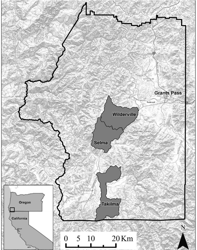
Figure 1. Map of study area with local population centers identified. The study sites are indicated as USGS hydrologic unit code 12 sub watersheds within Josephine County, southern Oregon. All wildlife cameras were contained within these three watersheds and are summarized at this scale to anonymize specific farm locations. From the top down, the sub watersheds are: Slate Creek, Lower Deer Creek, and Lower East Fork Illinois River. Map reproduced from Parker-Shames et al. 2020.
Wildlife camera surveys
We placed cameras on cannabis farms and in surrounding properties to capture a localized landscape gradient. The small-scale, private-land cannabis farms used in this study included one licensed recreational production site, one medically licensed (though non-compliant) production site, and six unlicensed sites. All farms were producing cannabis for sale, though in different markets depending on their access to licensed markets. We selected these eight cannabis farms because they: (1) were representative of the size and style of cultivation predominant in Josephine County in the years immediately following recreational legalization in 2015 (Parker-Shames et al. 2022; Parker-Shames et al. 2023), (2) were all established after recreational legalization except for the medical farm, (3) did not replace other plant-based agriculture, (4) granted us permission to set up cameras on site, and (5) were located next to a large section of unfarmed land (e.g., Bureau of Land Management, private, or timber lands) that could grant researchers access in order to place cameras across a gradient of distance to cannabis farms. Sampled farms were small (typically < 1 acre) and had been created by some form of clearing for production space. Three had constructed a fence or barrier around their crop. Specific land use practices and production philosophies differed among farms (e.g., pesticide use, type of fencing, presence of dogs, number of people working on the site, attitudes towards conservation). We cannot disclose precise farm locations, as per our research agreement for access.
Monitored farms were clustered within each watershed: one farm in Slate Creek, five in Lower Deer Creek, and two in Lower East Fork Illinois River; however, most farms were also located near other nearby cannabis farms that were not directly monitored in this study but were incorporated into covariate calculations (see Covariates below). We placed un-baited motion sensitive cameras (Bushnell E3, Bushnell Aggressor, or Moultriecam models) on cannabis farms as well as in random locations up to 1.5 km from the monitored farms. This is an expansion on previous camera research that only assessed on-site wildlife at these same farms (Parker-Shames et al., 2020). The surrounding context locations included private fields and trails, uncultivated spaces near non-cannabis gardens, private timber lands, outdoor recreational venues, and Bureau of Land Management lands. Randomized locations included three hemp fields next to cannabis farms. Hemp is the same species as cannabis but is regulated differently and in this region at the time of the study was produced in almost an identical fashion to cannabis, aside from typically using fewer fences. While we did not count these sites as cannabis themselves, they were located directly next to cannabis farms and so function similarly to them in the models as a low distance to cannabis.
We placed cameras approximately 0.5 m from the ground to capture animals roughly 1 kg and larger (e.g. squirrels). We set cameras to take bursts of 2 photos, with a quiet period of 15 seconds. To guide the placement of cameras, we overlaid the area surrounding each cannabis farm cluster with a grid of 50 x 50 m cells and then selected a random sample of at least one quarter of grid cells (a minimum of 45 stations in each watershed). We selected a 50 x 50 m cell size because we wanted to be able to detect fine scale space use responses of wildlife. The random sample was stratified by vegetation openness and distance to cannabis farm in all watersheds, and additionally by distance to clearcut in the Slate Creek watershed, such that cameras were placed in proportion to the landscape attributes and a distance gradient was achieved. When a selected site was inaccessible, we selected a new one that met the same stratification criteria. We rotated 15-20 cameras through the sampled grid cells more or less continuously from July 2018 – September 2019, ensuring each camera was deployed for at least one round of two-week duration. Because of rotations and field constraints, all cannabis sites were not monitored at the same time or for the same length of time (one to six rounds, with on-farm cameras monitored the most intensively) but each watershed was sampled for at least two different seasons. Altogether, we monitored a total of 149 camera stations for a combined 6,545 trap nights. We then employed a team of researchers trained to identify wildlife found in the study area to catalog photos by species.
Covariates
We calculated spatial and descriptive covariates to use in the SSOMs and MSDOMs (here we present them by data format and processing method but see Table 1 and Analyses below for specific assignment in modeling processes). We selected a primary covariate that addressed our main question of interest (i.e., the influence of cannabis production on wildlife), as well as covariates that might explain general space use, space use intensity, or detection patterns. We chose not to include characteristics about individual farms, which vary in their particular agricultural practices, as the focus of the study was to understand the effect of small-scale cannabis farms in the aggregate on wildlife.
First, we calculated spatial distance covariates from each site. Our main covariate of interest was distance to cannabis farms. To calculate distance to cannabis, we used the location data for participating farms in our study and augmented them with mapped data on Josephine County cannabis farms from 2016 aerial imagery so that distance to cannabis would not be limited to only participating farms (Parker-Shames et al. 2022). We then calculated the minimum Euclidean distance from each camera to its nearest cannabis farm using the package sf (Pebesma 2018) (v. 1.0.6) in R (R v. 2021-11-08 “Ghost Orchid”) (R Core Team 2021) using Rstudio (v. 2021.09.1 + 372) (Rstudio Team 2021). We transformed distance to cannabis using a square root to help fit potential thresholds in wildlife responses. Next, we again used the sf package, this time to calculate the distance from each camera to the nearest paved road, using this as a proxy for overall human impacts since in our study areas, human development and activity was concentrated along paved roads.
For our two raster-based covariates, we used the raster (Hijmans 2022) (v. 3.5.15), and exactextractr (Baston 2021) (v. 0.7.2) packages in R. We calculated the proportion of forested land cover within a 50 m buffer around each camera and extracted the elevation in meters at each camera site to capture topographic and vegetation features that often influence animal habitat (Reilly et al., 2017).
We also included non-spatial covariates in our analyses. We generated mean activity indices for dogs and humans by calculating the number of observations of humans or dogs, respectively, at each camera within the previous three days, divided by the number of days the camera was active. We chose an interval of three days to capture a time period that might reasonably affect wildlife while balancing data needs. This produced an activity rate where the beginning or end of placement rounds were on the same relative scale as all other days, and allowed us to examine the influence of dog and human activity (which was not limited to cannabis farms) directly across sites. We also included a covariate for Julian date of each interval, as well as Julian date squared, to capture seasonal peaks. We then included an estimated distance at which a camera could still detect an animal (generally lower in dense vegetation and higher in open sites), which was measured at camera setup.
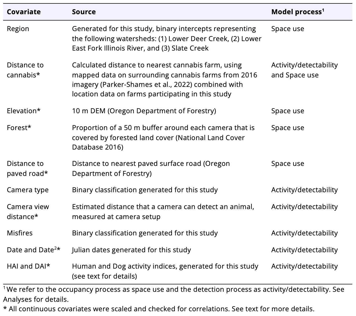
Table 1. Covariates used for SSOMs and MSDOMs.
All continuous variables were scaled so that they centered on 0 with a standard deviation of 1 (though Date2 was not scaled again after squaring Date) and checked for correlations (Pearson’s correlation, r<0.6) in R.
Finally, we used additional categorical covariates to account for potential effects of geographic region and camera function. Each camera was in one of three regions based on USGS Hydrologic Unit 12 watersheds, such that Region1 represents Lower Deer Creek, Region2 for Lower East Fork Illinois River, and Region3 for Slate Creek. We created a binary variable for camera type. We gave a 0 to camera models that generally performed well in our study system (Bushnell Aggressors) and a 1 to older models (Bushnell E3s and Moultriecams). We also assigned a binary code based on the number of misfires (inadvertent camera triggers with no animal in the frame, usually the result of waving vegetation) that occurred at each placement, because a high misfire rate indicated that cameras might be more likely to miss an animal moving in front of it. We assigned cameras with a low number of misfires (<20 over the two-week placement) a 0, and those with a high misfire rate (>20) a 1, based on the natural break in the data.
Analyses
We assessed the local space use of wildlife in response to cannabis production using single-season site occupancy models, SSOMs. We then examined how cannabis production influences wildlife nocturnality by fitting multi-state diel models, MSDOMs. The use of occupancy models to assess space use is becoming more common in wildlife response studies, as even traditional uses of occupancy modeling are influenced by wildlife space use (Neilson et al. 2018; Nickel et al. 2020). However, typical of most camera-based studies, our application of occupancy models knowingly violates several assumptions of traditional occupancy models: first, because cameras were spaced relatively close together compared to the home range of species included in the study, we have likely violated the assumption of independent cameras (i.e. spatial sampling units); second, as a result of the aforementioned spacing as well as sampling across two years (which was long enough that individuals may move in and out of the study area), we likely violated the model’s assumption of geographic and demographic closure (Mackenzie et al. 2006). We have done our best to account for violations in closure assumptions by using a narrow interval of replication (24 hours), which should minimize animal movement during closed periods (see Single species models below). We also include regional fixed effects to partially account for potential geographic dependencies between cameras. Ultimately, our interest was in space use associations and not estimates of occupancy, and we believe outstanding violations will have little bearing on our results.
We interpret occupancy for the models as space use rather than true occupancy (and therefore refer to it as “space use”). We operationalize detection as a combination of intensity of use, and camera detectability or error (which we refer to as “activity/detectability”). Estimating space use (the probability that the animal uses the site at any point during the study period) rather than occupancy means we do not make an assumption that sites are truly closed. We then interpret the activity/detectability probability as a combination of the probability that the species is detected and the intensity of use of the site within its larger range (Burton et al. 2015; Neilson et al. 2018; Stewart et al. 2018). This interpretation is common in camera-based studies (e.g. Nickel et al. 2020; Suraci et al. 2021). We proceed while being careful to acknowledge where appropriate that any covariate’s influence on activity/detectability probability is a combination of its effect on detection and the intensity with which an animal uses a given space. In addition, we have taken care to include variables in the activity/detectability process to account for what we anticipate to be the largest sources of variation in detectability, so that the other variables should primarily influence detections via their effects on space use intensity.
Note that we include distance to cannabis in both space use and activity/detectability processes in our models. Because we are using these processes to examine two different facets of animal behavior—space use and space use intensity—including our covariate of interest in both processes allows us to examine differing types of behavioral responses to disturbance within the same model. It is common to include covariates in both submodels in a variety of occupancy modeling approaches, as the model’s hierarchical structure allows for the effects of covariates on detection and occupancy to be estimated separately.
Site occupancy models
Our first main objective was to examine animals’ space use in relation to distance from cannabis farms. To do so, we conducted SSOM analyses on 13 wild and one domestic species (see provided data) (MacKenzie et al., 2002). We summarized species observations on and surrounding cannabis farms and created detection histories (i.e., tables where a “1” indicated the species was photographed at a given camera station during the respective 24-hr time interval when the camera was active in a given round, a “0” that it was not, and an “NA” for inactive periods between sampling rounds) using the package CamtrapR (CamtrapR v. 2.0.3) (Niedballa et al. 2016) in program R. We used a 24-hr time interval because our focus was on estimating space use associations instead of occupancy (see Analyses above), and a short interval reduced the likelihood of the same individual animal being detected on neighboring cameras (Latif, Ellis, and Amundson 2016; Steenweg et al. 2018).
We modeled the space use probabilities of the most commonly detected wild species and one domestic species, including: black bear (Ursus americanus), black-tailed deer (Odocoileus hemionus), bobcat (Lynx rufus), coyote (Canis latrans), gray fox (Urocyon cinereoargenteus), black-tailed jackrabbit (Lepus californicus), raccoon (Procyon lotor), striped skunk (Mephitis mephitis), California ground squirrel (Otospermophilus beecheyi), gray squirrel (Sciurus griseus), wild turkey (Meleagris gallopavo), California quail (Callipepla californica), mountain quail (Oreortyx pictus), and domestic dog (Canis lupus familiaris) using the NIMBLE and nimbleEcology packages in Program R (de Valpine et al. 2017; Goldstein et al. 2020). We selected these species because they had sufficient detections to model (see provided data), and because they covered a range of functional groups, including predators and mesopredators (bear, coyote, bobcat, gray fox, raccoon), omnivores (bear, gray fox, striped skunk, raccoon), large and small prey (deer, jackrabbit, squirrels, turkey, quails), and a domestic predator (dog). We included dogs as an added check on our modeling approach, as their general distributions and associations are already well known in the study system, unlike wildlife species.
We modeled the observed data (ys) as a binary variable where 1 was an observation for a given species at camera station s, and 0 was a non-detection. We modeled the observed data for each species, denoted ys~ Bern(zs, ps), as a product of both true space use (zs; occurrence) of a given species at a site and our probability of actually detecting it (ps), which is also influenced by intensity of use at a given site. The model assumes that true space use is an outcome of a Bernoulli-distributed random variable, denoted zs~ Bern(Psis), where Psis is the probability that a given species used site s on any day during the survey period.
We assumed that cannabis production might influence the activity/detectability and space use of each species differently. For space use, we expected that increasing distance from cannabis farms would increase animal space use (i.e., due to avoidance of cannabis farms) for all species except domestic dogs. We also expected that elevation and forested land cover would influence space use based on their importance in other wildlife studies (e.g., Reilly et al., 2017). We expected proximity to paved roads to negatively affect space use, and to function as a proxy for other non-cannabis forms of human land use, including residences, in our study system. Finally, we accounted for potential regional differences in the three watersheds by including a fixed effect of region (parameterized as region-specific intercepts). Therefore, we constructed the space use submodel as follows:
Equation 1.
Where I(RegionX[s]) is an indicator variable equal to 1 if site s is in Region X, and 0 otherwise, Cannabis is the square root of distance to cannabis, Elevation is the elevation in meters at the camera site, Forest is the proportion of area around each camera site that is forested within a 50 m buffer, and Roads is the distance from the nearest paved roadway. All continuous variables were scaled.
For activity/detectability, we expected that increasing distance from cannabis farms would increase intensity of use (e.g., due to temporal avoidance on farms leading to lower activity rates closer to cannabis) for all species except domestic dogs. Separately from the general influence of cannabis farms themselves, we expected increased recent activity rate of dogs and humans to decrease intensity of use for all wild species (Nickel et al. 2020; Reilly et al. 2017). We further expected time of the year to influence intensity of use, based on seasonal changes in activity patterns (Furnas and McGrann 2018). Finally, we expected that the camera model, view distance (how far the camera can detect an animal), and number of misfires of each camera setup might influence its ability to detect animals. Therefore, we constructed the activity/detectability submodel as:
Equation 2.
Where Cannabis is the square root of distance to cannabis, HAI and DAI are activity indices for humans and dogs respectively, Date is the julian date, Date2 is the julian date squared, Type is a binary grouping of camera type, View is the estimated distance at which a camera can still detect an animal, and Misfires is the number of misfires. All continuous variables were scaled.
We fit our models using a Bayesian Markov-chain Monte Carlo (MCMC) method in R using the NIMBLE and nimbleEcology packages (de Valpine et al., 2017; Goldstein et al., 2020). We used weakly informative prior distributions (normal distributions with mean 0 and standard deviation 5) for all space use and activity/detectability parameters (Gelman et al. 2008). Space use and activity/detectability parameters were calculated from three chains run for 10,000 iterations, with a burn in of 200 and thinned by 1. We assessed model convergence by examining trace plots and R-hat values (<1.1) for parameter estimates. We considered parameter estimates as meaningful (i.e. the Bayesian analogue of “significant”) when their 95% credible interval did not overlap zero.
We evaluated model fit using posterior predictive checks. Looping over MCMC iterations with a thinning interval of 20, we simulated a new dataset from the model based on that iteration’s parameter values and calculated the deviance of the full model for the simulated dataset. We then compared the posterior mean deviance of the model estimated with the true data to the distribution of simulated deviances and calculated a Bayesian p-value as the fraction of simulated deviances greater than the posterior mean deviance. If this p-value was outside the interval (0.05, 0.95), this indicates that the observed value was extreme relative to expectations based on model structure, which we interpret as evidence of poor model fit.
Multi-state diel models
Our second major objective was to examine animals’ temporal activity patterns and degree of nocturnality in relation to distance from cannabis farms. Following Rivera et al. (2022), we estimated multi-state diel occupancy models (MSDOMs) (Appendix Table 1). We modeled the diel occupancy probabilities of the following species: black bear, black-tailed deer, bobcat, coyote, gray fox, black-tailed jackrabbit, raccoon, striped skunk, and domestic dog using the NIMBLE package in R. For the MSDOMs, we excluded squirrels, turkey, and quail, because they are primarily diurnal species.
The MSDOM extends the site occupancy model, replacing the binary occupancy (present/not present) and detection (observed/not observed) states with a multi-state framework representing nighttime and daytime use. The MSDOM considers nighttime and daytime occupancy separately, allowing covariates to influence occupancy differently during the night and day. For each site, we constructed a multi-state detection history as follows. In each 24-hour observation period at each site, a species was assigned one of four detection states indicating whether the species was: (1) not observed at all, (2) only observed during the day, (3) only observed at night, or (4) observed both during the day and at night. Multi-state detections are categorically distributed as:
Equation 3.
where detection probabilities are determined based on the latent state zi. This latent state is itself categorically distributed as
Equation 4.
where ψi is a vector of length 4 where the nth element, ψi,n, gives the probability that the true occupancy state of site i is n. Mirroring the detection states, there are four true occupancy states: (1) the site is not occupied by the species, (2) the site is occupied by the species only during the day, (3) the site is occupied by the species only at night, and (4) the site is occupied by the species during both the day and night. The multi-state occupancy probabilities ψi are associated with covariates using a multinomial logit link, as
Equation 5.
where xi is a vector of site-level covariates influencing occupancy, βNight are coefficients representing the effect of each covariate in xi on nighttime occupancy, and βDay are the effect coefficients of those covariates on daytime occupancy. The vector xi contained the same covariates used in the site occupancy models previously (Eqn. 1).
The 4×4 detection matrix P was parameterized following Equation 3 in Rivera et al. (2022). Briefly, daytime and nighttime probabilities are each associated with covariates as
Equation 6.
where pijDay is the probability that the species is detected only during the day given that it only occupies the site during the day, and is linked to daytime coefficients αDay and a vector of covariates wij influencing detection, and equivalently for nighttime detection. Then, the elements of the detection matrix are
Equation 7.
The multistate diel occupancy formulation can be used to compute an index of nocturnality at a given site
Equation 8.
which can be interpreted as the probability that the species occupies site i only at night, given that it is present. Values of θi closer to 1 indicate the model prediction that the species uses the site strictly at night, while values close to 0 correspond to a species using the site strictly during the day. As in the SSOM, we interpret camera-level occupancy as space use and detection probabilities as incorporating both imperfect detection probabilities and intensity of use.
We aim to investigate whether a species’ nocturnality varies with distance to cannabis. This corresponds to the derivative of θi with respect to distance to cannabis, dθ/dc, which is a deterministic function of the daytime and nighttime effects of cannabis on occupancy and a given distance to cannabis, c (see Appendix S2 for the full equation and derivation). This value depends on the level of c, though not on the level of other covariate data. For each species, we obtain posterior distributions of dθ/dc for levels of c representing distances of 0 m, 100 m, and 1000 m from cannabis. If the 95% credible interval of at least one of these quantities did not contain zero, we interpreted that as evidence that proximity to cannabis influences the degree to which the species uses space nocturnally.
We fit MSDOMs for each of nine species in NIMBLE using 3 chains of 10,000 iterations with a burn-in period of 200 samples. We used weakly informative priors (normal distributions with mean 0 and standard deviation 2.5) for all detection and occupancy parameters. For all species, all stochastic nodes had an effective sample size of at least 190 and a Gelman-Rubin diagnostic of at most 1.06. For each species, we interpret the posterior distributions of dθ/dc and make predictions of nocturnality over a grid of distances to cannabis for visualization. We evaluated model fit using posterior predictive checks as for SSOMs.
Results
We detected 41 individual non-human species and species groupings (e.g., “rodents”) for a total of 20,083 detections. We mainly detected common species such as black-tailed deer, jackrabbit, squirrels, gray fox, turkey, coyote, etc., as well as domestic animals such as dogs, cats, and horses (see provided data). However, we did document other more elusive species such as ringtail (Bassariscus astutus) and spotted skunk (Spilogale gracilis), as well as a single sighting of a porcupine (Erethizon dorsatum) and a fisher. We detected humans more frequently than any domestic or wild animal, particularly on and surrounding cannabis farms. The number of wild species detected at least once at each site was relatively evenly spread across the gradient of distances to cannabis farms and the species we selected for modeling were detected relatively frequently and on at least 10% of cameras, aside from bobcats, raccoons, and California quail, which were detected on at least 6% of cameras (see provided data).
Site occupancy models
For the SSOMs, space use and activity/detectability varied by species (Appendix Table 1, Fig. 2). Recall that for our models, we interpreted occupancy as space use, and activity/detectability as a combination of detectability and space use intensity (see Analyses above) (Nickel et al., 2020; Suraci et al., 2021). Six species had a meaningful space use response to cannabis farms (i.e., their 95% credible interval for distance to cannabis did not overlap zero). Deer, raccoon, California quail, and mountain quail space use probability increased with distance from cannabis farms, indicating potential avoidance. Domestic dogs, as expected, decreased in predicted space use with distance to cannabis farms. Interestingly, gray fox space use probability also decreased with distance from cannabis farms, indicating that these species may be more likely to be found on and around cannabis farms (Fig. 2).
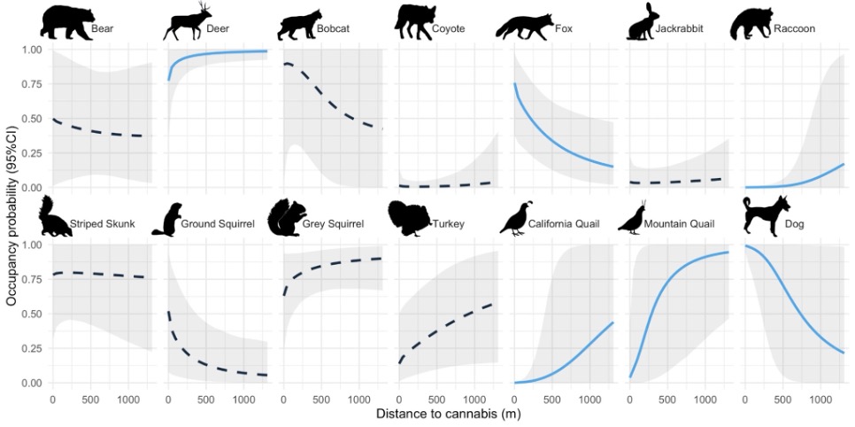
Figure 2. Predicted space use probabilities of each single species model to the covariate for distance from cannabis farms. Probabilities correspond to Region 1 with all other covariates held at mean conditions. The species with solid lines in blue (deer, gray fox, ground squirrels, tree squirrels, and domestic dogs) all had a credibly non-zero response (the 95% credible interval of the coefficient representing the effect of cannabis on space use did not overlap zero). The gray regions represent the 95% credible intervals for the estimated probabilities, but note that credible intervals for predicted space use probabilities are not the same as credible intervals for the parameter estimates themselves, and incorporate uncertainty in the intercept as well as the relationship between distance to cannabis and space use (see Appendix Table 1 for parameter-specific uncertainties). Animal silhouettes from phylopic.org (Mountain Quail by Dr. Palomo-Munoz).
Seven species had a statistically meaningful activity/detectability response to cannabis farms (Appendix Table 1, Fig. 3). As expected, deer and ground squirrel activity/detectability probability increased with distance from cannabis farms, indicating that they used areas further from cannabis farms more intensively. For ground squirrels, this means that although they did not seem to avoid cannabis farms, they may use the spaces farther from farms more intensively. Again as expected, domestic dog activity/detectability probability decreased with distance from cannabis farms, confirming that they spent most of their time on and surrounding cannabis farms, though overall activity/detectability was low. Surprisingly however, jackrabbit, raccoon, California quail, and mountain quail activity/detectability also decreased with distance from cannabis farms. As a reminder, given our modeling approach, frequent activity/detectability on occupied cannabis farms means that these species also likely have used the space on and surrounding cannabis farms more intensively (Fig. 3).
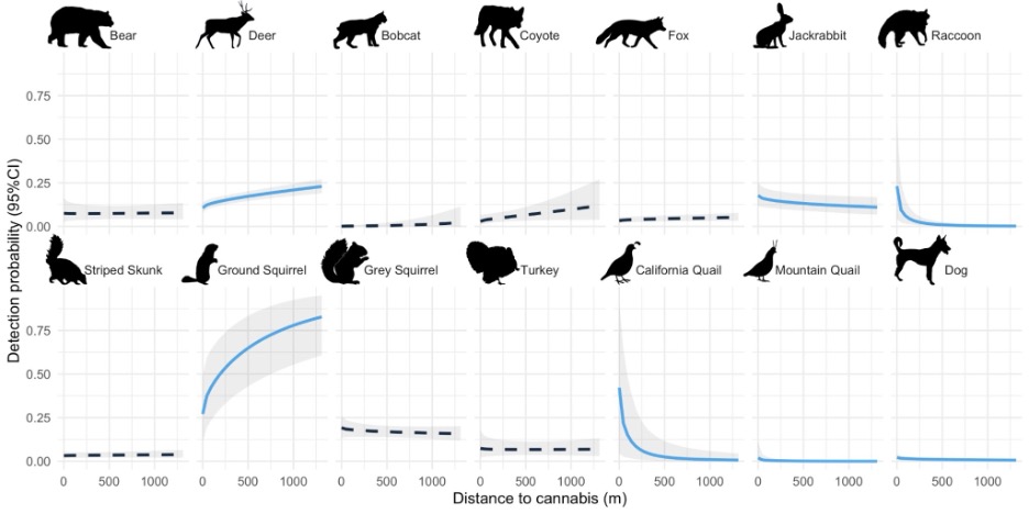
Figure 3. Predicted activity/detectability response of each single species model to the covariate for distance from cannabis farms. Probabilities correspond to Region 1 with all other covariates held at mean conditions. The species with solid lines in blue (deer, bobcat, jackrabbit, striped skunk, ground squirrel, and domestic dog) all had a credibly non-zero response (the 95% credible interval of the coefficient representing the effect of cannabis on activity/detectability did not overlap zero). The gray regions represent the 95% credible interval for the estimated probability, but note that credible intervals for predicted space use probabilities are not the same as credible intervals for the parameter estimates themselves, and incorporate uncertainty in the intercept as well as the relationship between distance to cannabis and activity/detectability (see Appendix Table 1 for parameter-specific uncertainties). Animal silhouettes from phylopic.org (Mountain Quail by Dr. Palomo-Munoz).
The other model covariates aside from cannabis cultivation also varied by species (Appendix Table 1). For all species except bobcats, at least one regional intercept was meaningfully associated with space use probability. Elevation predicted space use for gray squirrels, ground squirrels, turkeys, and striped skunks. Forest proportion predicted space use for jackrabbits, tree squirrels, ground squirrels, and dogs. Paved roads predicted space use for gray squirrels, California quail, and dogs. All activity/detectability covariates were meaningful for at least some species. All species had at least one credibly non-zero covariate for detectability, which included camera type, view distance, and misfires. There was evidence for seasonal effects, with date and date2 meaningfully predicting activity/detectability for half of the study species. The activity indices had meaningful, and somewhat surprising results. Bobcats were negatively associated with human activity, and gray squirrel activity/detectability was negatively associated with dog activity. However, deer, jackrabbit, and striped skunk activity/detectability probabilities were all positively associated with human activity, while bobcat, coyote, gray fox, and jackrabbit activity/detectability probabilities were all positively associated with dog activity.
Multi-species diel models
For the MSDOMs, six species meaningfully altered their nocturnality in response to distance from cannabis farms (Fig. 4). Bear and deer nocturnality decreased with distance to cannabis farms, indicating that they were most nocturnal on and surrounding cannabis farms. Bobcat, gray fox, jackrabbit, and dog nocturnality all increased with distance to cannabis farms, indicating that their activity patterns on and surrounding cannabis farms were more diurnal. While point estimates of nocturnality were imprecise due to difficulty in estimating the intercept (Fig. 4), our derivative-based approach to assessing change in nocturnality with respect to distance to cannabis allowed us to assess the relationship with confidence.
Across all MSDOMs and SSOMs, Bayesian p-values generated from posterior predictive checks were within the interval (0.5, 0.95), indicating no evidence of poor model fit.
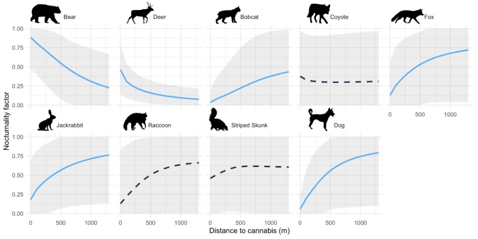
Figure 4. Predicted nocturnality response of each single species diel model to the covariate for distance from cannabis farms. Probabilities correspond to Region 1 with all other covariates held at mean conditions. The species with solid lines in blue (bear, deer, bobcat, fox, jackrabbit, dog) all had a credibly non-zero response (the 95% credible interval of the relationship between distance to cannabis and nocturnality did not overlap zero). The gray bars represent the 95% credible interval for the estimated probability. Note that credible intervals for predicted nocturnality probabilities at particular distances are wide, as they incorporate uncertainty in the intercept (see Appendix Table 1 for parameter-specific uncertainties), and determination of nonzero slopes was based on the estimate of the derivative of nocturnality with respect to cannabis use. Animal silhouettes from phylopic.org (Mountain Quail by Dr. Palomo-Munoz).
Discussion
This study assessed wildlife space use and temporal responses to active small-scale outdoor cannabis farms on private land. Our work provides a timely baseline for understanding potential wildlife community consequences from an emerging land use frontier. Our application of occupancy modeling to space use responses and diel patterns has yielded two main conclusions: 1) even at small scales, rural cannabis farming can affect local wildlife behavior; 2) patterns of animal responses are species-specific, but generally fall into three categories: avoidance, attraction, or mixed response (Fig. 5). These results have implications for the cannabis industry and small farm strategies for conservation. For example, our results could help inform state cannabis regulations or criteria for wildlife-conscious farming certifications.
Cannabis production comes in many forms in different locations, and this study does not represent all of them. This study is most applicable for small-scale and mixed light outdoor cannabis cultivation occurring on private lands in legacy production regions of the rural Western US. It is very likely that larger farms would have a greater impact on wildlife than those included in this study, or that farms developed in areas with existing agriculture might have less, or different kinds of effects. Similarly, this was an early snapshot of wildlife responses to disturbance, which might change over time. Because cannabis production is often unique from other forms of agriculture, these types of observational studies are valuable and merit repeating in different contexts.
Overall cannabis farm effects
Eight out of 14 species modeled using SSOMs had a meaningful response to distance from cannabis farms, either in space use or activity/detectability, and 6 of 9 species in the MSDOMs meaningfully changed in nocturnality in response to distance from cannabis farms. Our hypothesis that a majority of species would avoid farms was not supported, since the strength and direction of effects were species-specific. However, the results imply a general ability for cannabis farming to affect local wildlife space use and activity patterns. The relationships between space use and activity/detectability probabilities and distance to cannabis also indicate that there could be threshold effects relatively close to farms where the slope of the relationship is steeper (Fig. 2; Fig. 3), though further steps would be needed to confirm this relationship.
The variation in our results are in contrast with research from the western US on vineyards and avocado production that indicated that wildlife used farmed land in seeming preference over surrounding land uses (Hilty and Merenlender 2004; Nogeire et al. 2013). However, these other studies were conducted in areas where the agricultural land formed a corridor through more human-dominated land covers, which is the inverse of the landscape studied here. Our results are similar to studies on agroforestry systems with annual and perennial croplands, where there may be differential responses to agricultural land use and potential for filtering responses (Brashares 2010; Ferreira et al. 2018).
Compared to the other covariates in the models, distance to cannabis farms meaningfully affected more species than any other covariate for space use. It was particularly surprising that wildlife responded to the physical land use of cannabis farms even more than human or dog activity, given that in other systems animal space use intensity often responds more to human activity than human footprint (Nickel et al. 2020), and is often negatively affected by the presence of dogs (Reilly et al., 2017). This implies that cannabis farms may combine multiple potential sources of disturbance that wildlife may react to, and/or that the physical modifications for cannabis farms on their own are enough to trigger wildlife responses. More research is needed to disentangle the effects of different types of grows (legal status, size, license type, etc.), the potential mechanistic pathways by which cannabis farms may affect wildlife, and how different land use practices on cannabis farms modify those impacts. Future studies isolating potential mechanisms of deterrence and attraction (e.g. fencing, light pollution, generator noise, dog/human residence, trash/compost storage, configuration of land clearing, etc.) would help elucidate some of the species-specific behaviors documented in this study.
Space use and temporal patterns
Overall, space use and temporal responses to cannabis were species-specific, confirming our alternative hypothesis for individual responses. While functional- or diet-group patterns are not as clear in this case as in other study systems (e.g., Rich et al. 2016; Ferreira et al. 2018), a few general patterns may be emerging as to overall types of responses (Fig. 5). Our approach of using an occupancy modeling framework to assess wildlife space use associations was useful to identify emerging patterns, because it allowed us to look at space use separately from inferences on space use intensity (although the latter is difficult to disentangle from detectability). Adding a specific analysis of nocturnality also allowed us to separately assess temporal partitioning. This is important because it helps capture different types of responses: attraction and deterrence, as well as potential behavioral shifts or mixed responses in activity patterns (Nickel et al., 2020; Neilson et al., 2018; Burton et al., 2015). For example, this helped identify opposing space use and activity/detectability responses in occupancy and nocturnality.
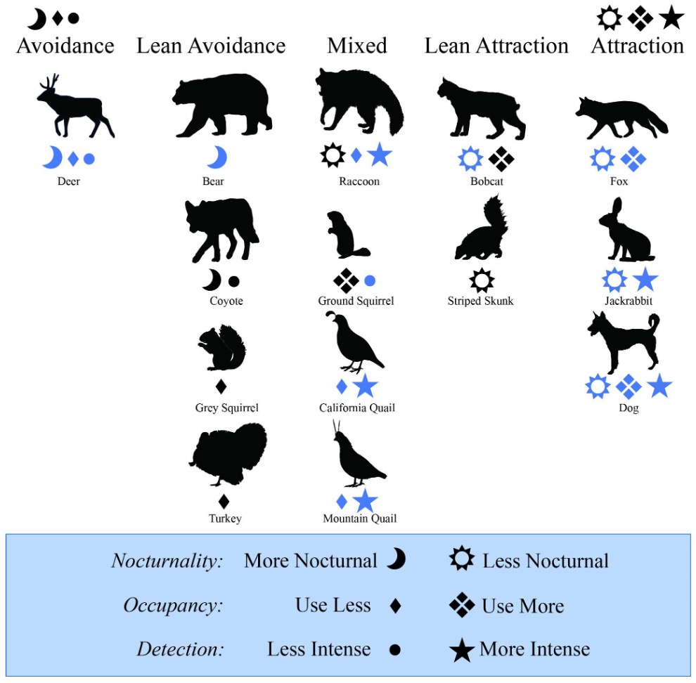
Figure 5. Visual summary of results, grouped by response type categories. Only results that trended towards a non-zero effect are represented. Symbols in blue represent credibly non-zero results. Species include deer, bear, coyote, gray squirrel, turkey, raccoon, ground squirrel, California quail, mountain quail, bobcat, striped skunk, gray fox, jackrabbit, and domestic dog. Animal silhouettes from phylopic.org (Mountain Quail by Dr. Palomo-Munoz).
Some species avoided cannabis by decreasing overall space use (i.e., occupancy, see Analyses) and activity/detectability (i.e., space use intensity and detectability) while increasing nocturnality near to cannabis farms (Fig. 5). Deer were the clearest example, responding in all three metrics; however, results for coyote, bear, turkey, and gray squirrels indicate they may also lean towards an avoidance response. These species may be physically blocked from areas close to cannabis farms by fencing, or they may be more sensitive to disturbance. The result is somewhat surprising given that many of these species have been associated with adaptation to human presence in other systems (Suraci et al. 2021).
On the other hand, several species demonstrated an attraction to cannabis by increasing space use and activity/detectability while decreasing nocturnality near to cannabis farms (Fig. 5). The clearest example of attraction was from domestic dogs, which was expected. Results for bobcats, gray foxes, jackrabbits, and striped skunks indicate they may also lean towards an attraction response. Most of the species demonstrating a potential attraction are mesopredators, which is consistent with other studies that demonstrate that these species are often behaviorally flexible and able to coexist in human-dominated spaces (Suraci et al., 2021; Nogeire et al., 2013). The pattern of mesopredator use of human spaces is also often explained via mesopredator release, when larger predators avoid an area of disturbance and thereby open a niche for smaller predators (Prugh et al., 2009). In this system, the larger predators might include bears or coyotes, which did not have a significant space use response though displayed other potential avoidance in space use intensity and nocturnality (Fig.5), or mountain lions (Puma concolor), which we were unable to model due to insufficient detections. However, all three of these large predators were photographed at least once in the middle of a cannabis farm (see provided data). For the only non-predator, jackrabbits, as well as the mesopredators, it may be that cannabis farms provide resources, or a predator shield effect (Berger 2007).
Finally, some species demonstrated a mixed response where decreased space use near cannabis farms was matched with increased activity/detectability (Fig. 5). This behavioral pattern was shared by California quail and mountain quail, as well as raccoons which also demonstrated potential decreased nocturnality near to farms. For these species, the combination of opposing behavioral responses indicates that while they generally avoid cannabis farms in space, the few areas that they do use, they may use more intensively, and/or less furtively during daylight hours. If this pattern is indeed driven by space use intensity, there are many possible explanations—for instance, perhaps these species, in an attempt to avoid cannabis farms, end up concentrated in smaller areas. One species, the ground squirrel, indicated an opposite response of a trend towards spatial attraction but a decreased space use intensity (Fig. 5). This inverted response suggests that while ground squirrels might be attracted to cannabis farms, they use spaces nearby less intensively. This makes sense as ground squirrels are sometimes crop pests (including for cannabis), and so may adjust their behavioral patterns to become more furtive to avoid removal (Hammond et al. 2019). It is interesting to note that aside from raccoons, the species that demonstrated mixed responses in space use and space use intensity were all diurnal species. Further research could examine whether this behavioral tradeoff is influenced by the limited ability of these species to shift their diel patterns (Gaynor et al. 2018).
Separately from these three general categories of response, it also appears that there could be a relationship between animal body size and temporal response. The species that tended to use sites near cannabis more during nocturnal periods, bear and deer, are also the largest species we modeled, while smaller bodied species like gray foxes or rabbits used sites near cannabis less during nocturnal periods. This is consistent with other diel pattern research that has indicated larger bodied species may trend towards being more sensitive to human disturbance (Gaynor et al. 2018). There could also be an effect of scale for these larger animals or wide ranging species like coyotes and bobcats, whose home ranges can extend farther than the areas under study and might influence their mechanisms of response to cannabis farms.
Conclusions
The results of our study hold implications for conservation and cannabis. We find evidence for on-site overlap between small-scale outdoor cannabis farms and local wildlife. The association of higher space use and space use intensity of many species on or near cannabis farms suggests that some animals may be using the farms regularly for rest and forage. The co-occurrence of wildlife with cannabis production emphasizes the importance of best management practices on-site for cannabis farms to ensure that this overlap does not result in harm to wildlife. There is an opportunity for future research to study the long-term population effects on wildlife that share space with cannabis production. While some research suggests that farmers perceive local wildlife as part of their environmental stewardship towards the land, not all farmers are likely to share the same view, and many farmers may lack resources or knowledge of wildlife conscious farming practices (Parker-Shames et al. 2023). It is also important to acknowledge that some of this wildlife overlap may not be beneficial for farmers. Some of the species with higher space use or activity/detectability rates close to farms, such as ground squirrels, quail, or raccoons, may also cause crop or property damage for farmers. Balancing coexistence with livelihoods will be as important for the cannabis industry as it is with any small-scale agriculture seeking to minimize local impacts (Crespin & Simonetti, 2019).
On the other hand, our results also demonstrate a broad ability for cannabis agriculture to influence local wildlife. While the implied indirect effects from cannabis farming on wildlife are, by and large, not extreme, it emphasizes the importance of land use planning for cannabis development, as even small disturbances in relatively undeveloped rural areas may influence local wildlife communities. This is valuable information, as efforts to formulate appropriate regulation, best management practices, or wildlife friendly certifications for cannabis are still ongoing. More research is needed on this rapidly changing agricultural frontier, but we hope that our research here may offer insights into an ecologically uncertain industry.
Finally, our novel approach of applying fine scale wildlife space use and temporal activity modeling to evaluate animal responses to disturbance is broadly relevant beyond cannabis agriculture. The combination of assessing space use, space use intensity, and nocturnality provides a detailed set of information to separate out and categorize different wildlife responses, all from a single data collection method of wildlife cameras. Our approach is also easily modifiable and allows researchers to incorporate different categories (e.g. crepuscular response), covariates, and scales. This innovative modeling technique not only enhances our understanding of wildlife behavior but also provides valuable insights for informing conservation and management strategies across various ecosystems.
Acknowledgments
We are deeply grateful for the farms that agreed to participate in this study; we know it took an inordinate amount of trust. Thank you also to all the landowners that agreed to let us set cameras on their properties. For indispensable support in the field, we thank our assistants, Christy Dunn and Maelagh Baker, as well as those who volunteered time in the field including Dylan Beal, Ron Raven, Bill Gray, and Amy Van Scoyoc. Thank you to the Brashares Lab for your consistent support and feedback, particularly Lindsey Rich for advice on study design. This project would not have been possible without the many undergraduate research assistants at UC Berkeley who helped sort photos: Alice Hua, Augie Clements, Jordan Pulaski, Theo Snow, Chloe Tilton, Elise Allen, Ellie Resendiz, Emily Ohman, Haina Jin, Hannah Liu, Jessica Stubbs, Julianna Sams, Michael Xiao, Sapphire Suzuki, Sara Soderberg, Sasha Kozlov, Tiffany Chen, Cece Gonzalez, and Varsha Madapoosi. Thank you to the Undergraduate Research Assistantship Program and Sponsored Projects for Undergraduate Research programs at UC Berkeley for providing student support and compensation, and to our funders, the Oliver Lyman Award for Summer Research and the NSF Graduate Research Fellowship Program. Finally, thank you to Dr. Gabriella Palomo for creating a beautiful mountain quail silhouette for us on phylopic.org.
Author Contributions
Phoebe Parker-Shames: conceptualization, data curation, formal analysis, funding acquisition, investigation, methodology, project administration, supervision, software, visualization, writing
Ben Goldstein: data curation, formal analysis, methodology, software, validation, visualization, writing
Justin Brashares: conceptualization, funding acquisition, methodology, supervision
Data Availability
All data from this study are provided here.
Supplemental Information
Supplemental Information can be found here.
Transparent Peer Review
Results from the Transparent Peer Review can be found here.
Recommended Citation
Parker-Shames, P., Goldstein, B.R., & Brashares, J.S. (2024). Spatial and temporal activity of wildlife on and surrounding cannabis farms. The Stacks: 24003. https://doi.org/10.60102/stacks-24003
References
Alberti, Marina, Eric P. Palkovacs, Simone Des Roches, Luc De Meester, Kristien I. Brans, Lynn Govaert, Nancy B. Grimm, et al. 2020. “The Complexity of Urban Eco-Evolutionary Dynamics.” BioScience 70 (9): 772–93. https://doi.org/10.1093/biosci/biaa079.
Arcview Market Research. 2016. “Executive Summary: The State of Legal Marijuana Markets, 4th Edition.” San Fransisco: Arcview Market Research. arcviewmarketresearch.com.
Atwood, Todd C., Harmon P. Weeks, and Thomas M. Gehring. 2004. “Spatial Ecology of Coyotes Along a Suburban-To-Rural Gradient.” Journal of Wildlife Management 68 (4): 1000–1009. https://doi.org/10.2193/0022-541x(2004)068[1000:seocaa]2.0.co;2.
Baston, Daniel. 2021. “Exactextractr: Fast Extraction from Raster Datasets Using Polygons.” https://CRAN.R-project.org/package=exactextractr.
Berger, J. 2007. “Fear, Human Shields and the Redistribution of Prey and Predators in Protected Areas.” Biology Letters 3 (6): 620–23. https://doi.org/10.1098/rsbl.2007.0415.
Borine, Roger. 1983. Soil Survey of Josephine County, Oregon. US Department of Agriculture, Soil Conservation Service. https://books.google.com/books?hl=en&lr=&id=jlIXF6Im160C&oi=fnd&pg=PP6&dq=rainfall+josephine+county+oregon&ots=AsXjPaQNuY&sig=w8cwKTTLW_RFlVzfM0lJMxwnN7Q#v=onepage&q=rainfall josephine county oregon&f=false.
Brashares, Justin S. 2010. “Filtering Wildlife.” Science 329 (5990): 402–3. https://doi.org/10.1126/science.1190095.
Burton, A. Cole, Eric Neilson, Dario Moreira, Andrew Ladle, Robin Steenweg, Jason T. Fisher, Erin Bayne, and Stan Boutin. 2015. “Wildlife Camera Trapping: A Review and Recommendations for Linking Surveys to Ecological Processes.” Journal of Applied Ecology 52 (3): 675–85. https://doi.org/10.1111/1365-2664.12432.
Butsic, Van, and Jacob C Brenner. 2016. “Cannabis (Cannabis Sativa or C. Indica) Agriculture and the Environment: A Systematic, Spatially-Explicit Survey and Potential Impacts.” Environmental Research Letters 11: 044023. https://doi.org/10.1088/1748-9326/11/4/044023.
Butsic, Van, Jennifer Carah, Matthias Baumann, Connor Stephens, and Jacob C Brenner. 2018. “The Emergence of Cannabis Agriculture Frontiers as Environmental Threats.” Environmental Research Letters 13: 124017. https://doi.org/10.1088/1748-9326/aaeade.
Carah, Jennifer K., Jeanette K. Howard, Sally E. Thompson, Anne G. Short Gianotti, Scott D. Bauer, Stephanie M. Carlson, David N. Dralle, et al. 2015. “High Time for Conservation: Adding the Environment to the Debate on Marijuana Liberalization.” BioScience 65 (8): 822–29. https://doi.org/10.1093/biosci/biv083.
Chouvy, Pierre-Arnaud. 2019. “Cannabis Cultivation in the World: Heritages, Trends and Challenges.” EchoGéo, no. 48 (July). https://doi.org/10.4000/echogeo.17591.
Corva, Dominic. 2014. “Requiem for a CAMP: The Life and Death of a Domestic U.S. Drug War Institution.” International Journal of Drug Policy 25 (1): 71–80. https://doi.org/10.1016/j.drugpo.2013.02.003.
Crespin, Silvio J., and Javier A. Simonetti. 2019. “Reconciling Farming and Wild Nature: Integrating Human–Wildlife Coexistence into the Land-Sharing and Land-Sparing Framework.” Ambio 48 (2): 131–38. https://doi.org/10.1007/s13280-018-1059-2.
Dillis, Christopher, Van Butsic, Diana Moanga, Phoebe Parker‐Shames, Ariani Wartenberg, and Theodore E. Grantham. 2022. “The Threat of Wildfire Is Unique to Cannabis among Agricultural Sectors in California.” Ecosphere 13 (9). https://doi.org/10.1002/ecs2.4205.
Estes, James, John Terborgh, and JS Brashares. 2011. “Trophic Downgrading of Planet Earth.” Science 333 (6040): 301–6. https://doi.org/10.1126/science.1205106.
Ferreira, Aluane S., Carlos A. Peres, Juliano André Bogoni, and Camila Righetto Cassano. 2018. “Use of Agroecosystem Matrix Habitats by Mammalian Carnivores (Carnivora): A Global-Scale Analysis.” Mammal Review 48 (4): 312–27. https://doi.org/10.1111/mam.12137.
Fidino, Mason, Travis Gallo, Elizabeth W. Lehrer, Maureen H. Murray, Cria A.M. Kay, Heather A. Sander, Brandon MacDougall, et al. 2021. “Landscape-Scale Differences among Cities Alter Common Species’ Responses to Urbanization.” Ecological Applications 31 (2): 1–12. https://doi.org/10.1002/eap.2253.
Frey, Sandra, J. P. Volpe, N. A. Heim, J. Paczkowski, and J. T. Fisher. 2020. “Move to Nocturnality Not a Universal Trend in Carnivore Species on Disturbed Landscapes.” Oikos 129 (8): 1128–40. https://doi.org/10.1111/oik.07251.
Frid, Alejandro, and Lawrence M. Dill. 2002. “Human-Caused Disturbance Stimuli as a Form of Predation Risk.” Conservation Ecology 6 (1): art11. https://doi.org/10.5751/ES-00404-060111.
Furnas, Brett J., and Michael C. McGrann. 2018. “Using Occupancy Modeling to Monitor Dates of Peak Vocal Activity for Passerines in California.” The Condor. https://doi.org/10.1650/CONDOR-17-165.1.
Gabriel, Mourad W., Leslie W. Woods, Robert Poppenga, Rick A. Sweitzer, Craig Thompson, Sean M. Matthews, J. Mark Higley, et al. 2012. “Anticoagulant Rodenticides on Our Public and Community Lands: Spatial Distribution of Exposure and Poisoning of a Rare Forest Carnivore.” PLoS ONE 7 (7): e40163. https://doi.org/10.1371/journal.pone.0040163.
Gabriel, Mourad W., Leslie W. Woods, Greta M. Wengert, Nicole Stephenson, J. Mark Higley, Craig Thompson, Sean M. Matthews, et al. 2015. “Patterns of Natural and Human-Caused Mortality Factors of a Rare Forest Carnivore, the Fisher (Pekania Pennanti) in California.” PLoS ONE 10 (11): e0140640. https://doi.org/10.1371/journal.pone.0140640.
Gallo, Travis, Mason Fidino, Brian Gerber, Adam A Ahlers, Julia L Angstmann, Max Amaya, Amy L Concilio, et al. 2022. “Mammals Adjust Diel Activity across Gradients of Urbanization.” ELife 11 (March): e74756. https://doi.org/10.7554/eLife.74756.
Gaynor, Kaitlyn M, Cheryl E Hojnowski, Neil H Carter, and Justin S Brashares. 2018. “The Influence of Human Disturbance on Wildlife Nocturnality.” Science 360 (6394): 1232–35.
Gelman, Andrew, Aleks Jakulin, Maria Grazia Pittau, and Yu-Sung Su. 2008. “A Weakly Informative Default Prior Distribution for Logistic and Other Regression Models.” The Annals of Applied Statistics 2 (4). https://doi.org/10.1214/08-AOAS191.
Goldstein, Benjamin R., Daniel Turek, Lauren C. Ponisio, and Perry de Valpine. 2020. “NimbleEcology: Distributions for Ecological Models in Nimble.” https://cran.r-project.org/package=nimbleEcology.
Hammond, Talisin T, Minnie Vo, Clara T Burton, Lisa L Surber, Eileen A Lacey, and Jennifer E Smith. 2019. “Physiological and Behavioral Responses to Anthropogenic Stressors in a Human-Tolerant Mammal.” Edited by Loren Hayes. Journal of Mammalogy 100 (6): 1928–40. https://doi.org/10.1093/jmammal/gyz134.
Hijmans, Robert J. 2022. “Raster: Geographic Data Analysis and Modeling.” https://CRAN.R-project.org/package=raster.
Hilty, Jodi A., and Adina M. Merenlender. 2004. “Use of Riparian Corridors and Vineyards by Mammalian Predators in Northern California.” Conservation Biology 18 (1): 126–35. https://doi.org/10.1111/j.1523-1739.2004.00225.x.
Hinton, Joseph W., Frank T. Van Manen, and Michael J. Chamberlain. 2015. “Space Use and Habitat Selection by Resident and Transient Coyotes (Canis Latrans).” PLoS ONE 10 (7): 1–17. https://doi.org/10.1371/journal.pone.0132203.
Klassen, Mark, and Brandon P. Anthony. 2019. “The Effects of Recreational Cannabis Legalization on Forest Management and Conservation Efforts in U.S. National Forests in the Pacific Northwest.” Ecological Economics 162: 39–48. https://doi.org/10.1016/j.ecolecon.2019.04.029.
Lark, Tyler J., Seth A. Spawn, Matthew Bougie, and Holly K. Gibbs. 2020. “Cropland Expansion in the United States Produces Marginal Yields at High Costs to Wildlife.” Nature Communications 11 (1): 1–11. https://doi.org/10.1038/s41467-020-18045-z.
Latif, Quresh S., Martha M. Ellis, and Courtney L. Amundson. 2016. “A Broader Definition of Occupancy: Comment on Hayes and Monfils.” Journal of Wildlife Management 80 (2): 192–94. https://doi.org/10.1002/jwmg.1022.
Levy, Sharon. 2014. “Pot Poisons Public Lands.” BioScience 64 (4): 265–71. https://doi.org/10.1093/biosci/biu020.
MacKenzie, Darryl I., James D. Nichols, Gideon B. Lachman, Sam Droege, Andrew A. Royle, and Catherine A. Langtimm. 2002. “Estimating Site Occupancy Rates When Detection Probabilities Are Less than One.” Ecology 83 (8): 2248–55. https://doi.org/10.1890/0012-9658(2002)083[2248:ESORWD]2.0.CO;2.
Mackenzie, D.I., J.D. Nichols, J.A. Royle, K.H. Pollock, L.L. Bailey, and J.E. Hines. 2006. Occupancy Estimation and Modeling: Inferring Patterns and Dynamics of Species Occurrence. Amsterdam: Elsevier.
Mendenhall, Chase D, Daniel S Karp, Christoph F J Meyer, Elizabeth A Hadly, and Gretchen C Daily. 2014. “Predicting Biodiversity Change and Averting Collapse in Agricultural Landscapes.” Nature 509. https://doi.org/10.1038/nature13139.
Muhly, Tyler B., Christina Semeniuk, Alessandro Massolo, Laura Hickman, and Marco Musiani. 2011. “Human Activity Helps Prey Win the Predator-Prey Space Race.” PLoS ONE 6 (3): 1–8. https://doi.org/10.1371/journal.pone.0017050.
Neilson, Eric W., Tal Avgar, A. Cole Burton, Kate Broadley, and Stan Boutin. 2018. “Animal Movement Affects Interpretation of Occupancy Models from Camera-Trap Surveys of Unmarked Animals.” Ecosphere 9 (1). https://doi.org/10.1002/ecs2.2092.
Nickel, Barry A., Justin P. Suraci, Maximilian L. Allen, and Christopher C. Wilmers. 2020. “Human Presence and Human Footprint Have Non-Equivalent Effects on Wildlife Spatiotemporal Habitat Use.” Biological Conservation 241 (August 2019): 108383. https://doi.org/10.1016/j.biocon.2019.108383.
Niedballa, Jürgen, Rahel Sollmann, Alexandre Courtiol, and Andreas Wilting. 2016. “CamtrapR: An R Package for Efficient Camera Trap Data Management.” Methods in Ecology and Evolution 7 (12): 1457–62. https://doi.org/10.1111/2041-210X.12600.
Nogeire, Theresa M., Frank W. Davis, Jennifer M. Duggan, Kevin R. Crooks, and Erin E. Boydston. 2013. “Carnivore Use of Avocado Orchards across an Agricultural-Wildland Gradient.” PLoS ONE 8 (7): 1–6. https://doi.org/10.1371/journal.pone.0068025.
Olson, David, Dominick a. DellaSala, Reed F. Noss, James R. Strittholt, Jamie Kass, Marni E. Koopman, and Thomas F. Allnutt. 2012. “Climate Change Refugia for Biodiversity in the Klamath-Siskiyou Ecoregion.” Natural Areas Journal 32 (1): 65–74. https://doi.org/10.3375/043.032.0108.
Olson, David M., Eric Dinerstein, Eric D. Wikramanayake, Neil D. Burgess, George V. N. Powell, Emma C. Underwood, Jennifer A. D’amico, et al. 2006. “Terrestrial Ecoregions of the World: A New Map of Life on Earth.” BioScience 51 (11): 933–38. https://doi.org/10.1641/0006-3568(2001)051[0933:teotwa]2.0.co;2.
Oregon Liquor Control Commission. 2019. “Marijuana License Applications as of 8:00 AM Monday, December 9, 2019.”
Padilla, Benjamin Juan, and Chris Sutherland. 2021. “Defining Dual-Axis Landscape Gradients of Human Influence for Studying Ecological Processes.” PLoS ONE 16 (11 November): 1–17. https://doi.org/10.1371/journal.pone.0252364.
Parker-Shames, Phoebe, Hekia Bodwitch, Justin S. Brashares, and Van Butsic. 2023. “Where Money Grows on Trees: A Socio-Ecological Assessment of Land Use Change in an Agricultural Frontier.” Landscape and Urban Planning 237 (September): 104783. https://doi.org/10.1016/j.landurbplan.2023.104783.
Parker-Shames, Phoebe, Christopher Choi, Van Butsic, David Green, Brent Barry, Katie Moriarty, Taal Levi, and Justin S. Brashares. 2022. “The Spatial Overlap of Small‐scale Cannabis Farms with Aquatic and Terrestrial Biodiversity.” Conservation Science and Practice 4 (2): 1–14. https://doi.org/10.1111/csp2.602.
Parker-Shames, Phoebe, Wenjing Xu, Lindsey Rich, and Justin S Brashares. 2020. “Coexisting with Cannabis: Wildlife Response to Marijuana Cultivation in the Klamath-Siskiyou Ecoregion.” California Fish and Wildlife 106 (2): 86–100.
Pebesma, Edzer. 2018. “Simple Features for R: Standardized Support for Spatial Vector Data.” R Journal 10 (1): 439–46. https://doi.org/10.32614/rj-2018-009.
Power, Mary E., David Tilman, James A. Estes, Bruce A. Menge, William J. Bond, L. Scott Mills, Gretchen Daily, Juan Carlos Castilla, Jane Lubchenco, and Robert T. Paine. 1996. “Challenges in the Quest for Keystones.” BioScience 46 (8): 609–20. https://doi.org/10.2307/1312990.
Prugh, Laura R., Chantal J. Stoner, Clinton W. Epps, William T. Bean, William J. Ripple, Andrea S. Laliberte, and Justin S. Brashares. 2009. “The Rise of the Mesopredator.” BioScience 59 (9): 779–91. https://doi.org/10.1525/bio.2009.59.9.9.
Reilly, M. L., M. W. Tobler, D. L. Sonderegger, and P. Beier. 2017. “Spatial and Temporal Response of Wildlife to Recreational Activities in the San Francisco Bay Ecoregion.” Biological Conservation 207: 117–26. https://doi.org/10.1016/j.biocon.2016.11.003.
Rich, Lindsey N., Ange Darnell Baker, and Erin Chappell. 2020. “Anthropogenic Noise: Potential Influences on Wildlife and Applications to Cannabis Cultivation.” California Fish and Wildlife 106 (2).
Rich, Lindsey N., David A.W. Miller, Hugh S. Robinson, J. Weldon McNutt, and Marcella J. Kelly. 2016. “Using Camera Trapping and Hierarchical Occupancy Modelling to Evaluate the Spatial Ecology of an African Mammal Community.” Journal of Applied Ecology 53 (4): 1225–35. https://doi.org/10.1111/1365-2664.12650.
Rich, L.N., E. Ferguson, A.D. Baker, and E. Chappell. 2020. “A Review of the Potential Impacts of Artificial Lights on Fish and Wildlife and How This May Apply to Cannabis Cultivation.” California Fish and Wildlife 106 (2).
Rich, L.N., S. McMillin, A.D. Baker, and E. Chappell. 2020. “Pesticides in California: Their Potential Impacts on Wildlife Resources and Their Use in Permitted Cannabis Cultivation.” California Fish and Wildlife 106 (2).
Ridout, M. S., and M. Linkie. 2009. “Estimating Overlap of Daily Activity Patterns from Camera Trap Data.” Journal of Agricultural, Biological, and Environmental Statistics 14 (3): 322–37. https://doi.org/10.1198/jabes.2009.08038.
Rindfuss, Ronald R., Barbara Entwisle, Stephen J. Walsh, Carlos F. Mena, Christine M. Erlien, and Clark L. Gray. 2007. “Frontier Land Use Change: Synthesis, Challenges, and next Steps.” Annals of the Association of American Geographers 97 (4): 739–54. https://doi.org/10.1111/j.1467-8306.2007.00580.x.
Rivera, Kimberly, Mason Fidino, Zach J. Farris, Seth B. Magle, Asia Murphy, and Brian D. Gerber. 2022. “Rethinking Habitat Occupancy Modeling and the Role of Diel Activity in an Anthropogenic World.” The American Naturalist 200 (4): 556–70. https://doi.org/10.1086/720714.
Rstudio Team. 2021. “RStudio: Integrated Development Environment for R.” Rstudio, PBC, Boston MA. http://www.rstudio.com.
Schmitz, Oswald J., Vlastimil Krivan, and Ofer Ovadia. 2004. “Trophic Cascades: The Primacy of Trait-Mediated Indirect Interactions.” Ecology Letters 7 (2): 153–63. https://doi.org/10.1111/j.1461-0248.2003.00560.x.
Smith, Vincent, Maud Powell, David Mungeam, and Regan Emmons. 2019. “Stakeholder Perceptions of the Impact of Cannabis Production on the Southern Oregon Food System.” Journal of Agriculture, Food Systems, and Community Development 8 (4): 1–11. https://doi.org/10.5304/jafscd.2019.084.012.
Steenweg, Robin, Mark Hebblewhite, Jesse Whittington, Paul Lukacs, and Kevin McKelvey. 2018. “Sampling Scales Define Occupancy and Underlying Occupancy–Abundance Relationships in Animals.” Ecology 99 (1): 172–83. https://doi.org/10.1002/ecy.2054.
Stewart, Frances E.C., Jason T. Fisher, A. Cole Burton, and John P. Volpe. 2018. “Species Occurrence Data Reflect the Magnitude of Animal Movements Better than the Proximity of Animal Space Use:” Ecosphere 9 (2). https://doi.org/10.1002/ecs2.2112.
Suraci, Justin P., Kaitlyn M. Gaynor, Maximilian L. Allen, Peter Alexander, Justin S. Brashares, Sara Cendejas-Zarelli, Kevin Crooks, et al. 2021. “Disturbance Type and Species Life History Predict Mammal Responses to Humans.” Global Change Biology 27 (16): 3718–31. https://doi.org/10.1111/gcb.15650.
Thompson, Craig, Richard Sweitzer, Mourad Gabriel, Kathryn Purcell, Reginald Barrett, and Robert Poppenga. 2014. “Impacts of Rodenticide and Insecticide Toxicants from Marijuana Cultivation Sites on Fisher Survival Rates in the Sierra National Forest, California.” Conservation Letters 7 (2): 91–102. https://doi.org/10.1111/conl.12038.
Valpine, Perry de, Daniel Turek, Christopher J. Paciorek, Clifford Anderson-Bergman, Duncan Temple Lang, and Rastislav Bodik. 2017. “Programming With Models: Writing Statistical Algorithms for General Model Structures With NIMBLE.” Journal of Computational and Graphical Statistics 26 (2): 403–13. https://doi.org/10.1080/10618600.2016.1172487.
Van Scoyoc, Amy, Justine A. Smith, Kaitlyn M. Gaynor, Kristin Barker, and Justin S. Brashares. 2023. “The Influence of Human Activity on Predator–Prey Spatiotemporal Overlap.” Journal of Animal Ecology 92 (6): 1124–34. https://doi.org/10.1111/1365-2656.13892.
Wang, Ian, Jacob C. Brenner, and Van Butsic. 2017. “The Expansion of an Emerging Agricultural Crop Threatens Deforestation and Fragmentation.” Frontiers in Ecology and Evolution 15 (9): 495–501. https://doi.org/10.1002/fee.1634.
Wang, Yiwei, Justine A. Smith, and Christopher C. Wilmers. 2017. “Residential Development Alters Behavior, Movement, and Energetics in an Apex Predator, the Puma.” PLoS ONE 12 (10): 1–17. https://doi.org/10.1371/journal.pone.0184687.
Wartenberg, Ariani C, Patricia A Holden, Hekia Bodwitch, Phoebe Parker-Shames, Thomas Novotny, Thomas C Harmon, Stephen C Hart, et al. 2021. “Cannabis and the Environment: What Science Tells Us and What We Still Need to Know.” Environmental Science and Technology Letters. https://doi.org/10.1021/acs.estlett.0c00844.
Wilkinson, Christine E., Alex McInturff, Jennifer R. B. Miller, Veronica Yovovich, Kaitlyn M. Gaynor, Kendall Calhoun, Harshad Karandikar, et al. 2020. “An Ecological Framework for Contextualizing Carnivore–Livestock Conflict.” Conservation Biology 34 (4): 854–67. https://doi.org/10.1111/cobi.13469.
Accepted by 5 of 5 reviewers
Open Access
Peer-Reviewed
Creative Commons
Submitted: 01 January 2024
Accepted: 10 June 2024
Published: 06 July 2024
Funding Information: This research was funded by the Oliver Lyman Award for Summer Research (UC Berkeley) and the NSF Graduate Research Fellowship Program.
Conflicts of Interest: The authors declare no conflicts of interest.
© 2024 Parker-Shames et al. The Stacks


